Chapter 6
Continuous Probability Distributions
Learning Objectives
1. Understand the difference between how probabilities are computed for discrete and continuous
random variables.
2. Know how to compute probability values for a continuous uniform probability distribution and be
able to compute the expected value and variance for such a distribution.
3. Be able to compute probabilities using a normal probability distribution. Understand the role of the
standard normal distribution in this process.
4. Be able to compute probabilities using an exponential probability distribution.
5. Understand the relationship between the Poisson and exponential probability distributions.
Solutions:
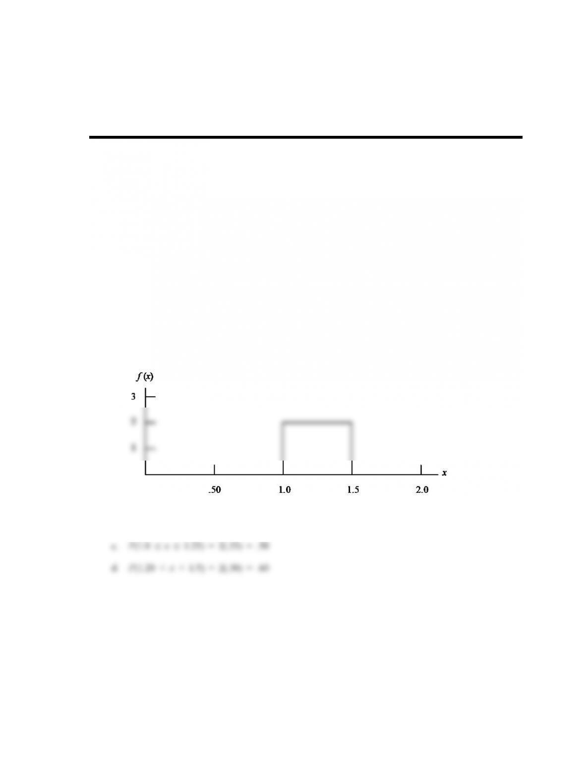
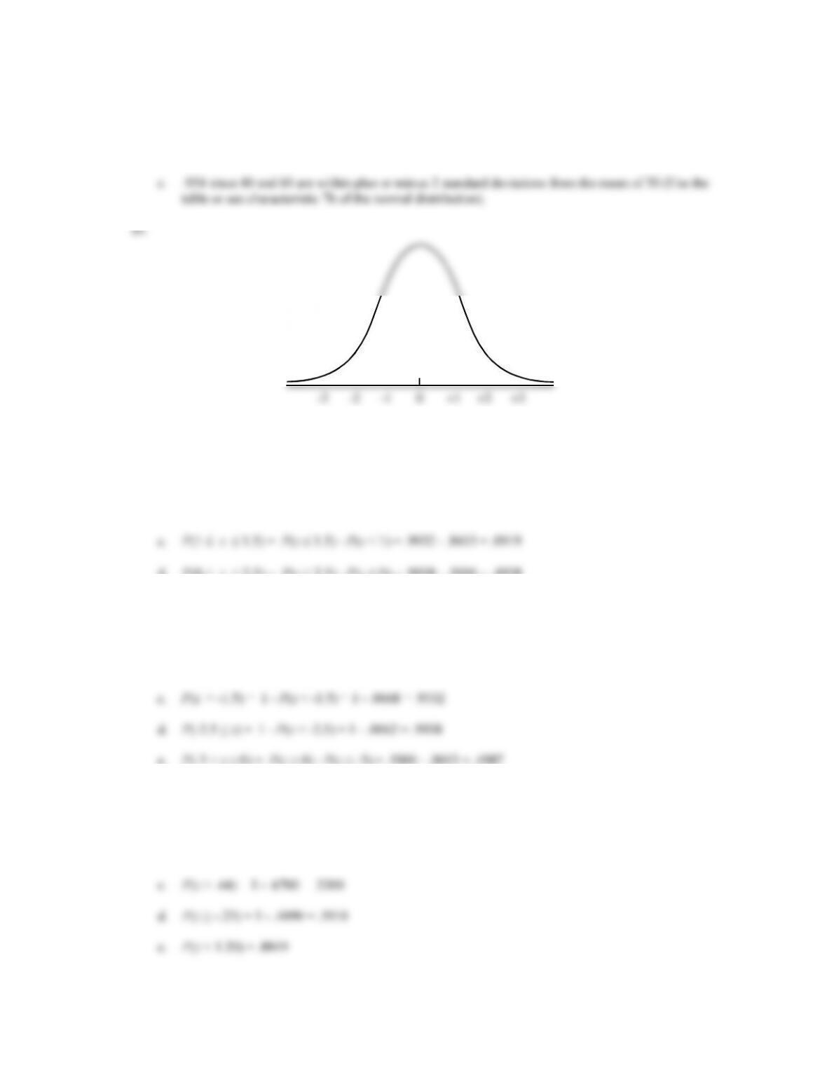
1. a.
b. P(x = 1.25) = 0. The probability of any single point is zero since the area under the curve above
any single point is zero.
2. a.
b. P(x < 15) = .10(5) = .50
c. P(12 x 18) = .10(6) = .60
10 20
12
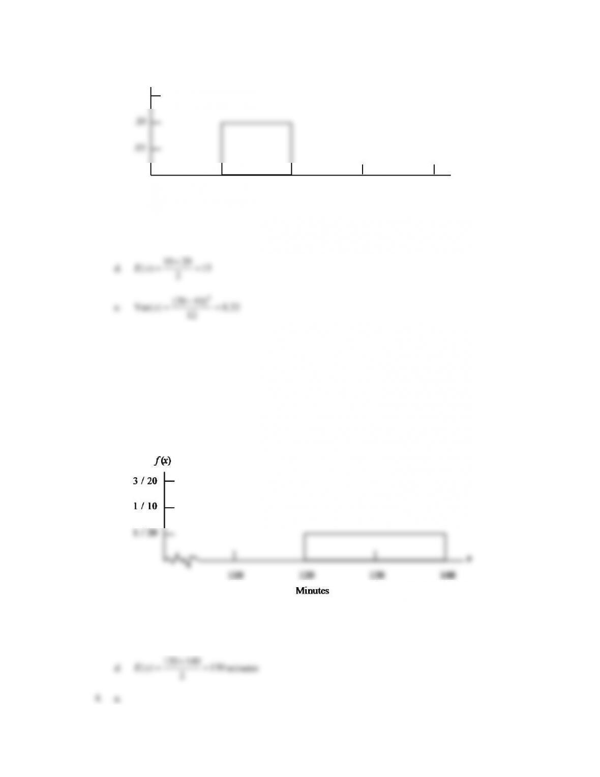
3. a.
b. P(x 130) = (1/20) (130 – 120) = 0.50
c. P(x > 135) = (1/20) (140 – 135) = 0.25
120 140
.15
.10
.05
10 20 30 40
f (x)
x
0
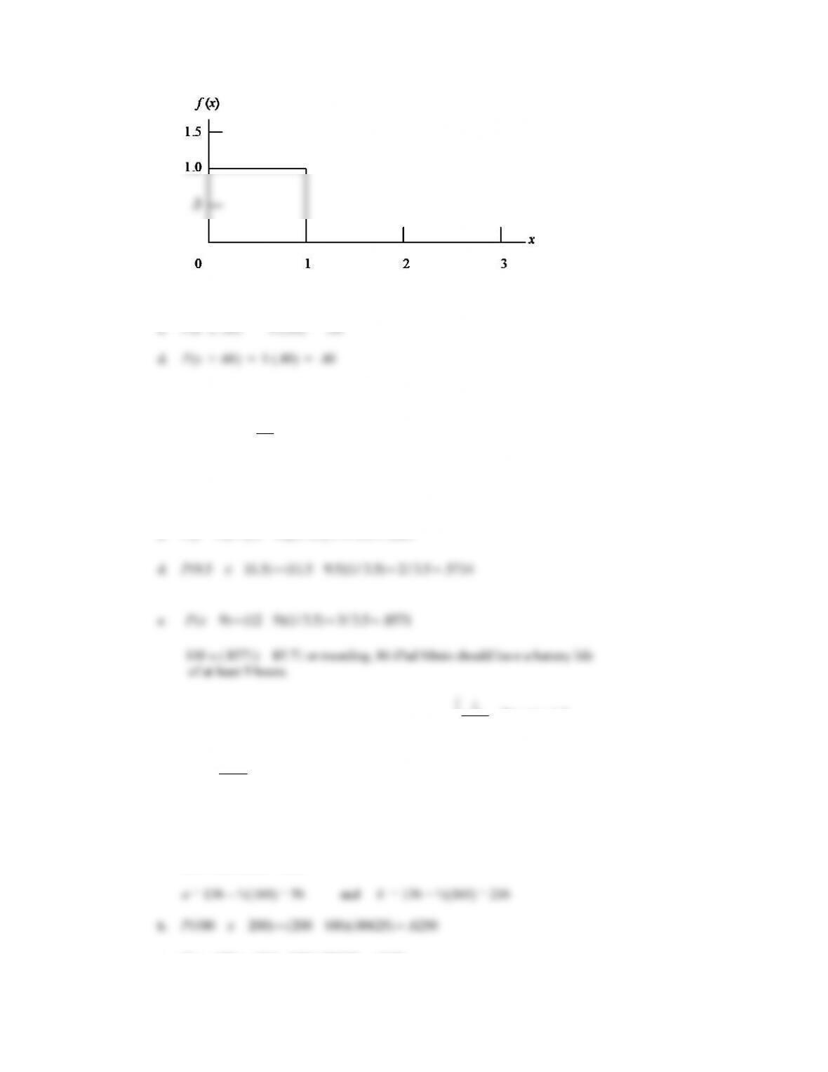
b. P(.25 < x < .75) = 1 (.50) = .50
c. P(x .30) = 1 (.30) = .30
5. a. Length of Interval = 12 – 8.5 = 3.5
f(x)=1
3.5 for 8.5 £x£12
0 elsewhere
ì
í
ï
î
ï
b.
P(x£10)=(10 –8.5)(1/ 3.5) =1.5/ 3.5 =.4286
c.
P(x³11)=(12 –11)(1/ 3.5) =1/ 3.5 =.2857
6. a. For a uniform probability density function
f(x)=1
b–a for a£x£b
0 elsewhere
ì
í
ï
î
ï
Thus,
1
b–a
= .00625.
Solving for
b–a
, we have
b–a
= 1/.00625 = 160
In a uniform probability distribution, ½ of this interval is below the mean and ½ of this interval is
above the mean. Thus,
c.
P(x³150) =(216–150)(.00625) =.4125
d.
P(x£80)=(80 –56)(.00625) =.1500
The probability your competitor will bid lower than you, and you get the bid, is .40.
b. P(10,000 x < 14,000) = 4000 (1 / 5000) = .80
c. A bid of $15,000 gives a probability of 1 of getting the property.
d. Yes, the bid that maximizes expected profit is $13,000.
The probability of getting the property with a bid of $13,000 is
P(10,000 x < 13,000) = 3000 (1 / 5000) = .60.
The probability of not getting the property with a bid of $13,000 is .40.
8.
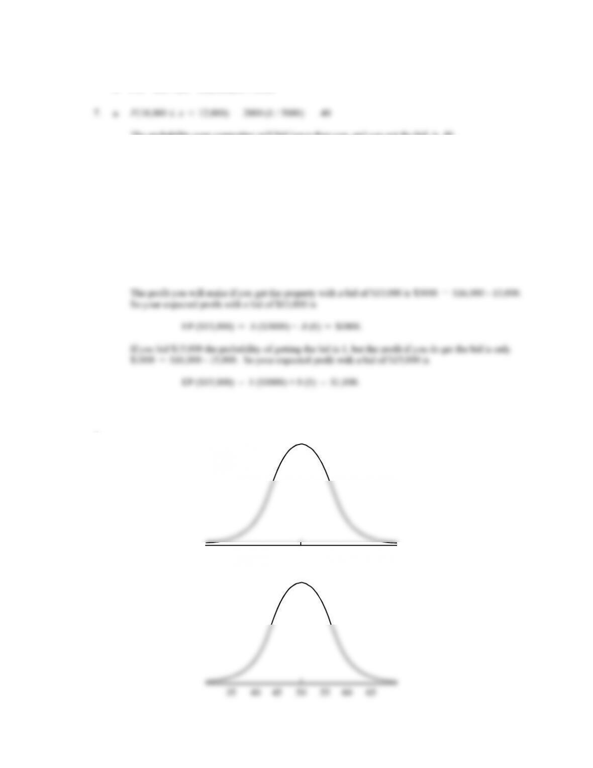
9. a.
50
= 5
s
35 40 45 55 60 65
100
= 10
s
70 80 90 110120130
b. .683 since 45 and 55 are within plus or minus 1 standard deviation from the mean of 50 (Use the
table or see characteristic 7a of the normal distribution).
These probabilities can be obtained using Excel’s NORM.S.DIST function or the standard normal
probability table in the text.
a. P(z 1.5) = .9332
b. P(z 1.0) = .8413
d. P(0 < z < 2.5) = P(z < 2.5) – P(z 0) = .9938 – .5000 = .4938
11. These probabilities can be obtained using Excel’s NORM.S.DIST function or the standard normal
probability table in the text.
a. P(z -1) = .1587
b. P(z ≥ -1) = 1 – P(z < -1) = 1 – .1587 = .8413
e. P(-3 < z ≤ 0) = P(z ≤ 0) – P(z ≤ -3) = .5000 – .0013 = .4987
12. These probabilities can be obtained using Excel’s NORM.S.DIST function or the standard normal
probability table in the text.
a. P(0 ≤ z ≤ .83) = .7967 – .5000 = .2967
b. P(-1.57 ≤ z ≤ 0) = .5000 – .0582 = .4418
0
-3 -2 -1 +1 +2 +3
13. These probabilities can be obtained using Excel’s NORM.S.DIST function or the standard normal
probability table in the text.
a. P(-1.98 z .49) = P(z .49) – P(z < -1.98) = .6879 – .0239 = .6640
14. These z values can be obtained using Excel’s NORM.S.INV function or by using the standard
normal probability table in the text.
a. The z value corresponding to a cumulative probability of .9750 is z = 1.96.
b. The z value here also corresponds to a cumulative probability of .9750: z = 1.96.
15. These z values can be obtained using Excel’s NORM.S.INV function or by using the standard
normal probability table in the text.
a. The z value corresponding to a cumulative probability of .2119 is z = –.80.
b. Compute .9030/2 = .4515; z corresponds to a cumulative probability of .5000 + .4515 = .9515. So z
= 1.66.
16. These z values can be obtained using Excel’s NORM.S.INV function or the standard normal
probability table in the text.
a. The area to the left of z is 1 – .0100 = .9900. The z value in the table with a cumulative probability
closest to .9900 is z = 2.33.
17.
= 385 and
s
= 110
a.
z=x–
m
s
=550–385
110 =1.50
(z£1.50)
b.
z=x–
m
s
=250–385
110 = –1.23
P
(x£250)
= P
(z£–1.23)
= .1093
c. For x = 500,
z=x–
m
s
=500–385
110 =1.05
For x = 300,
z=x–
m
s
=300–385
110 = –.77
P(300
£
x
£
400) = P
(z£1.05)
–
P
(z£–.77)
= .8531
–
.2206 = .6325
1–.03=.97
z=1.88
xz
s
=+
= 385 + 1.88(110) = $592
a. At x = 20,
20 14.4 1.27
4.4
z−
==
P(z 1.27) = .8980
4.4
P(z ≤ -1.00) = .1587
So, P(x 10) = .1587
x = 14.4 + 4.4(1.28) = 20.03
A return of 20.03% or higher will put a domestic stock fund in the top 10%
Using Excel: 1-NORM.INV(.9,14.4,4.4) = 20.0388
a.
500 328 1.87
92
x
z
s
−−
= = =
P(x > 500) = P(z > 1.87) = 1 – P(z ≤ 1.87) = 1 – .9693 = .0307
The probability that the emergency room visit will cost more than $500 is .0307.
92
s
P(x < 250) = P(z < -.85) = .1977
The probability that the emergency room visit will cost less than $250 is .1977.
92
s
For x = 300,
300 328 .30
92
x
z
s
−−
= = = −
P(300 < x < 400) = P(z < .78) – P(z < -.30) = .7823 – .3821 = .4002
The probability that the emergency room visit will cost between $300 and $400 is .4002.
xz
s
=+
= 328 – 1.41(92) = $198.28
For a patient to have a charge in the lower 8%, the cost of the visit must have been $198.28 or less.
Using Excel: NORM.INV(.08,328,92) = 198.73
P(z < -.92) = .1788
So, P(x < 3.50) = .1788
At x = 3.50,
3.50 3.40 .50
.20
z−
==
P(z < .50) = .6915
So, P(x < 3.50) = .6915
Using Excel: NORM.DIST(3.5,3.40,.20,TRUE) = .6915
5 8.35 1.34
2.5
x
z
s
−−
= = = −
P(5 ≤ x ≤ 10) = P(-1.34 ≤ z ≤ .66)= P(z ≤ .66) – P(z ≤ -1.34)
= .7454 – .0901
= .6553
x =
+ z
s
= 8.35 + 1.88(2.5) = 13.05 hours
Using Excel: NORM.INV(.97,8.35,2.5) = 13.0530
A household must view slightly over 13 hours of television a day to be in the top 3% of television
2.5
x
z
s
= = = −
Therefore 15.87% of students will not complete on time.
(60) (.1587) = 9.522
We would expect 9.522 students to be unable to complete the exam in time.
s
225 = –1.55
P
(x<400)
= P
(z<–1.55)
= .0606
The probability that expenses will be less than $400 is .0606.
Using Excel: NORM.DIST(400,749,225,TRUE) = .0604
(x³800)
(z³.23)
The probability that expenses will be $800 or more is .4090.
Using Excel: 1-NORM.DIST(800,749,225,TRUE) = .4103
m
For x = 500,
z=x–
m
s
=500–749
225 = –1.11
P(500
£
x
£
1000) = P
(z£1.12)
–
P
(z£–1.11)
= .8686
–
.1335 = .7351
The probability that expenses will be between $500 and $1000 is .7351.
Using Excel: NORM.DIST(1000,749,225,TRUE) – NORM.DIST(500,749,225,TRUE) = .7335
d. The upper 5%, or area =
1–.05=.95
occurs for
z=1.645
Using Excel: NORM.INV(.95,749,225) = 1119.0921