52. Excel’s MIN, QUARTILE.EXC, and MAX functions provided the following five-number
summaries:
AT&T
Sprint
T-Mobile
Verizon
Minimum
66
63
68
75
First Quartile
68
65
71.25
77
Median
71
66
73.5
78.5
Third Quartile
73
67.75
74.75
79.75
Maximum
75
69
77
81
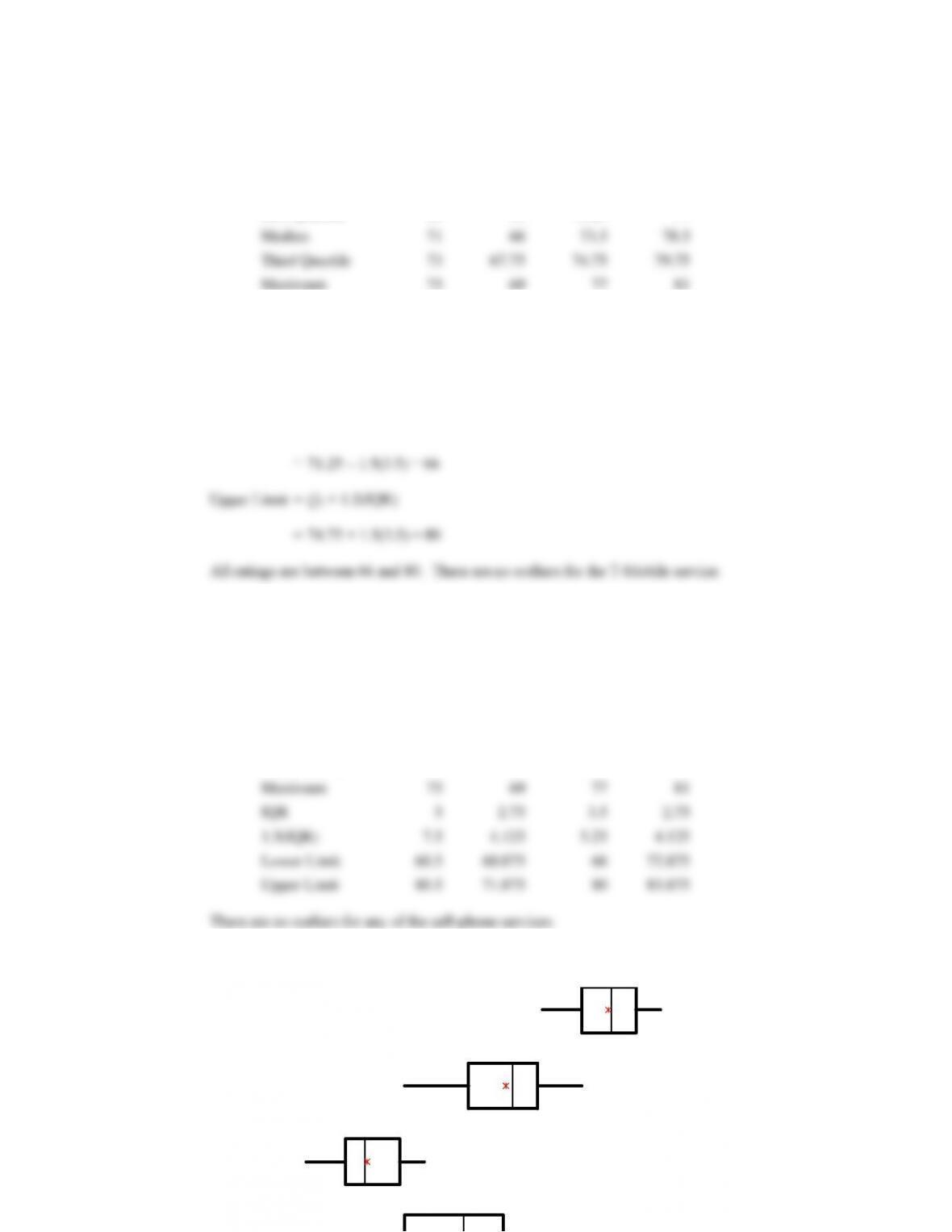
a. Median for T-Mobile is 73.5
b. 5- number summary: 68, 71.25, 73.5, 74.75, 77
c. IQR = Q3 – Q1 = 74.75 – 71.25 = 3.5
Lower Limit = Q1 – 1.5(IQR)
d. Using the five number summaries shown initially, the limits for the four cell-phone services are as
follows:
AT&T
Sprint
T-Mobile
Verizon
Minimum
66
63
68
75
First Quartile
68
65
71.25
77
Median
71
66
73.5
78.5
Third Quartile
73
67.75
74.75
79.75
Maximum
75
69
77
81
IQR
5
2.75
3.5
2.75
1.5(IQR)
7.5
4.125
5.25
4.125
Lower Limit
60.5
60.875
66
72.875
Upper Limit
80.5
71.875
80
83.875
There are no outliers for any of the cell-phone services.
e. A box plot created using StatTools follows.
Sprint
T-Mobile
Verizon
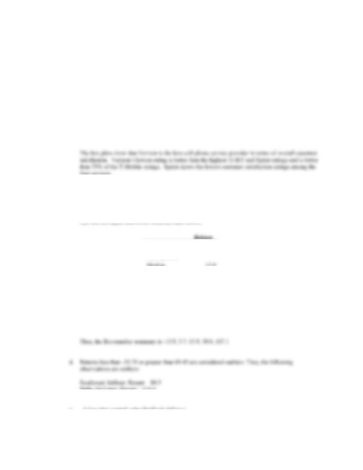
The box plots show that Verizon is the best cell-phone service provider in terms of overall customer
satisfaction. Verizon’s lowest rating is better than the highest AT&T and Sprint ratings and is better
than 75% of the T-Mobile ratings. Sprint shows the lowest customer satisfaction ratings among the
four services.
53. a. Using Excel’s MEDIAN function the median one year – total return is 13.9%.
b. 20 of the 50 companies or 40% had a one year – total return greater than the S&P average return.
c. Excel’s MIN, QUARTILE.EXC, and MAX functions provided the following results; values for the
IQR and the upper and lower limits are also shown.
Return
Minimum
-13.9
First Quartile
3.7
Median
13.9
Third Quartile
30.0
Maximum
117.1
IQR
26.3
1.5(IQR)
39.45
Lower Limit
-35.75
Upper Limit
69.45
Delta Air Lines: Return = 116.6
Facebook: Return = 117.1
e. A box plot created using StatTools follows:
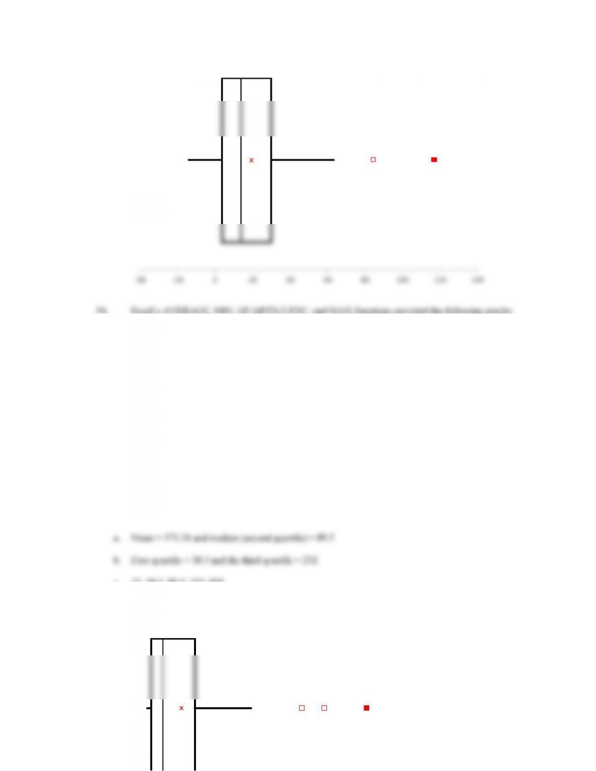
54. Excel’s AVERAGE, MIN, QUARTILE.EXC, and MAX functions provided the following results;
values for IQR and the upper and lower limits are also shown.
Personal Vehicles
(1000s)
Mean
173.24
Minimum
21
First Quartile
38.5
Second Quartile
89.5
Third Quartile
232
Maximum
995
IQR
193.5
1.5(IQR)
290.25
Lower Limit
-251.8
Upper Limit
522
c. 21, 38.5, 89.5, 232, 995
d. A box plot created using StatTools follows.
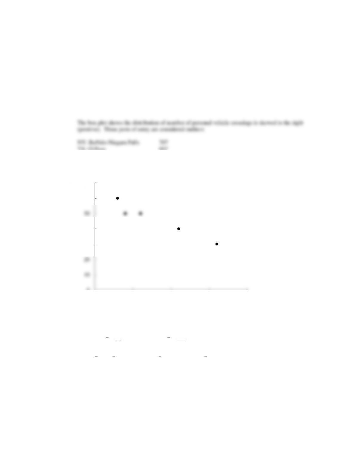
TX: El Paso 807
CA: San Ysidro 995
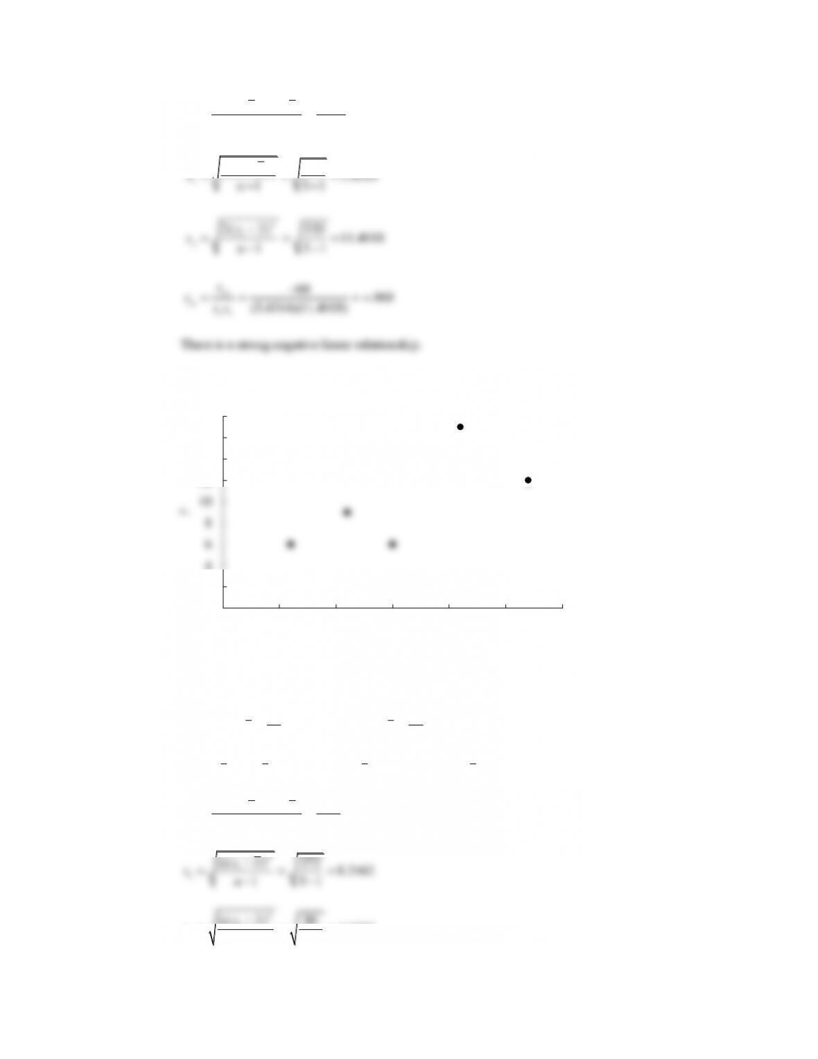
55. a.
b. Negative relationship
c/d.
x x y y
i i
= = = = = =40 40
58230 230
546
()( ) ( ) ( )x x y y x x y y
i i i i
− − = − − = − =240 118 520
2 2
0
10
20
30
40
50
60
70
0 5 10 15 20
y
x
2
2
( )( ) 240 60
1 5 1
() 118 5.4314
1 5 1
()520 11.4018
1 5 1
60 .969
(5.4314)(11.4018)
ii
xy
i
x
i
y
xy
xy
xy
x x y y
sn
xx
sn
yy
sn
s
rss
− − −
= = = −
−−
−
= = =
−−
−
= = =
−−
−
= = = −
There is a strong negative linear relationship.
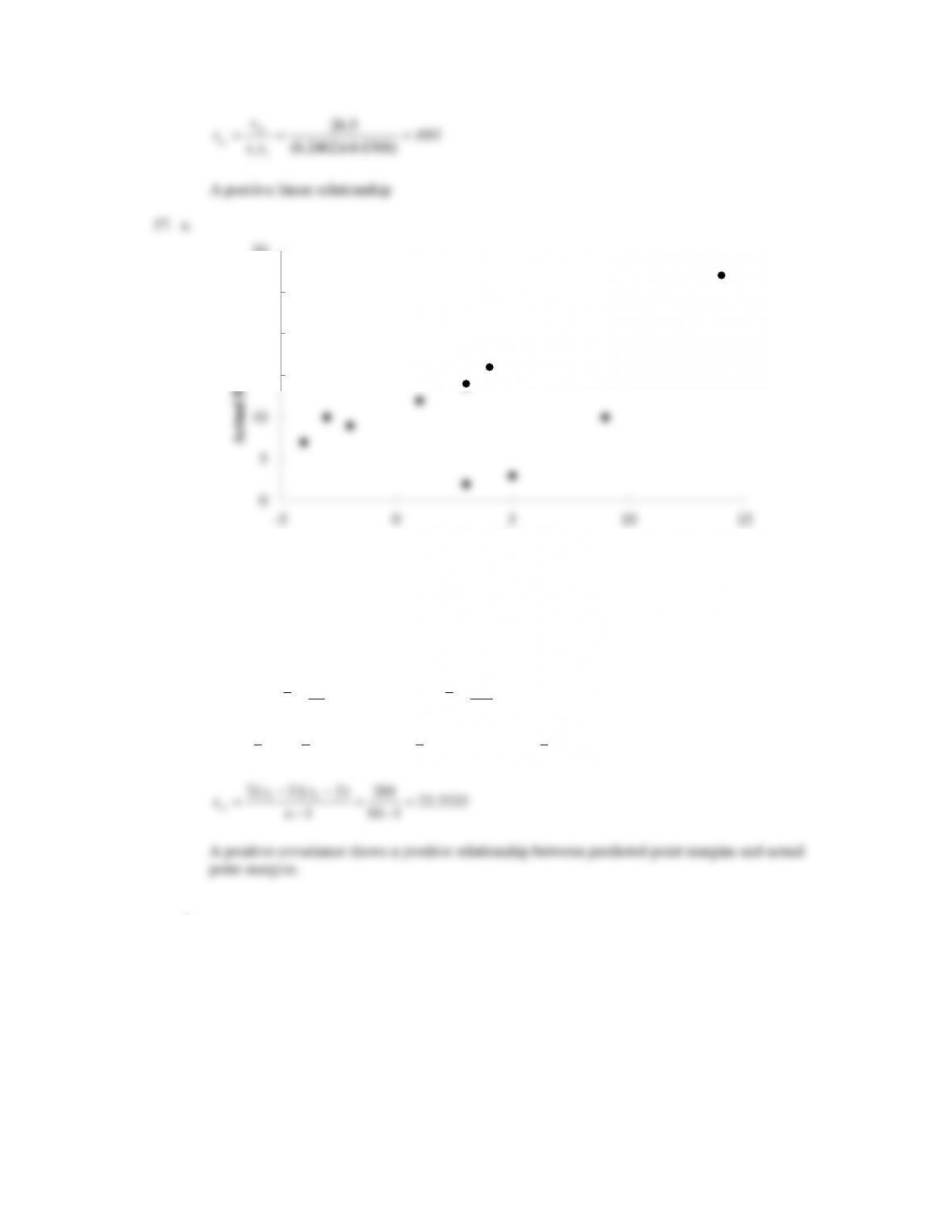
56. a.
b. Positive relationship
c/d.
x x y y
i i
= = = = = =80 80
516 50 50
510
()( ) ( ) ( )x x y y x x y y
i i i i
− − = − = − =106 272 86
2 2
( )( ) 106 26.5
1 5 1
ii
xy
x x y y
sn
− −
= = =
−−
2
() 272 8.2462
i
xx
−
0
2
4
6
8
10
12
14
16
18
0 5 10 15 20 25 30
y
x
26.5 .693
xy
s
b. The scatter diagram shows a positive relationship with higher predicted point margins associated
with higher actual point margins.
c. Let x = predicted point margin and y = actual point margin
30 110
30 3 110 11
10 10
ii
x x y y = = = = = =
22
( )( ) 201 ( ) 276 ( ) 458
i i i i
x x y y x x y y − − = − = − =
d.
0
5
10
15
20
25
30
-5 0 5 10 15
Actual Point Margin
Predicted Point Margin
2
2
() 276 5.5377
1 10 1
() 458 7.1336
1 10 1
22.3333 .565
(5.5377)(7.1336)
i
x
i
xy
xy
xy
xx
sn
yy
s
rss
−
= = =
−−
−
−−
= = =
The modest positive correlation shows that the Las Vegas predicted point margin is a general, but
not a perfect, indicator of the actual point margin in college football bowl games.
Note: The Las Vegas odds makers set the point margins so that someone betting on a favored team
has to have the team win by more than the point margin to win the bet. For example, someone
betting on Auburn to win the Outback Bowl would have to have Auburn win by more than five
58. Let x = miles per hour and y = miles per gallon
420 270
420 42 270 27
10 10
ii
x x y y = = = = = =
22
( )( ) 475 ( ) 1660 ( ) 164
i i i i
x x y y x x y y − − = − − = − =
2
( )( ) 475 52.7778
1 10 1
()1660 13.5810
1 10 1
ii
xy
i
x
x x y y
sn
xx
sn
− − −
= = = −
−−
−
= = =
−−

59. a.
184 6.81
27
i
x
xn
= = =
170.93 6.33
27
i
y
yn
= = =
8.3
9.24
2.9093
2.2058
8.4638
4.3208
7.5
4.40
-1.9307
0.4695
3.7278
-1.3229
7.1
6.91
0.5793
0.0813
0.3355
0.1652
6.8
5.57
-0.0148
-0.7607
0.0002
0.5787
0.0113
5.5
3.87
-1.3148
-2.4607
1.7287
6.0552
3.2354
7.5
8.42
2.0893
0.4695
4.3650
1.4315
5.8
4.07
-1.0148
-2.2607
1.0298
5.1109
2.2942
9.3
6.53
0.1993
6.1761
0.0397
0.4952
5.7
5.57
-1.1148
-0.7607
1.2428
0.5787
0.8481
7.3
6.99
0.4852
0.6593
0.2354
0.4346
0.3199
8.2
7.56
1.3852
1.2293
1.9187
1.5111
1.7028
7.1
12.11
0.2852
5.7793
0.0813
33.3998
1.6482
6.3
4.39
-0.5148
-1.9407
0.2650
3.7665
0.9991
6.6
4.78
-0.2148
-1.5507
0.0461
2.4048
0.3331
2
2
( )( ) 25.5517 .9828
1 26
()25.7741 .9956
1 26
()130.0594 2.2366
1 26
.9828 .4413
(.9956)(2.2366)
ii
xy
i
x
i
y
xy
xy
xy
x x y y
sn
xx
sn
yy
sn
s
rss
− −
= = =
−
−
= = =
−
−
= = =
−
= = =
i
x
i
y
()
i
xx−
()
i
yy−
2
()
i
xx−
2
()
i
yy−
( )( )
ii
x x y y−−
7.1
7.02
0.2852
0.6893
0.0813
0.4751
0.1966
5.2
5.31
-1.6148
-1.0207
2.6076
1.0419
1.6483
7.8
5.38
0.9852
-0.9507
0.9706
0.9039
-0.9367
7.8
5.40
0.9852
-0.9307
0.9706
0.8663
-0.9170
5.8
5.00
-1.0148
-1.3307
1.0298
1.7709
1.3505
6.2
5.78
-0.6148
-0.5507
0.3780
0.3033
0.3386
6.3
6.08
-0.5148
-0.2507
0.2650
0.0629
0.1291
7.0
10.05
0.1852
3.7193
0.0343
13.8329
0.6888
6.2
4.75
-0.6148
-1.5807
0.3780
2.4987
0.9719
5.5
7.22
-1.3148
0.8893
1.7287
0.7908
-1.1692
6.5
3.79
-0.3148
-2.5407
0.0991
6.4554
0.7999
6.0
3.62
-0.8148
-2.7107
0.6639
7.3481
2.2088
Total
25.77407
130.0594
25.5517
b.
60. a.
b. DJIA :
227.57 9.10
25
i
x
xn
= = =
2
()5672.61 15.37
( 1) 24
i
xx
sn
−
= = =
−
227.29 9.09
25
i
x
2
()7679.81 17.89
( 1) 24
i
xx
−
−
c.
263.611 .959
(15.37)(17.89)
xy
xy
xy
s
rss
= = =
d. Based on this sample, the two indexes are very similar. They have a strong positive correlation. The
variance of the Russell 1000 is slightly larger than that of the DJIA.
0.00
2.00
4.00
6.00
8.00
10.00
12.00
14.00
4 5 6 7 8 9 10
Delinquent Loans (%)
Jobless Rate (%)
-50.00
-40.00
-30.00
-20.00
-10.00
0.00
10.00
20.00
30.00
40.00
-40.00 -30.00 -20.00 -10.00 0.00 10.00 20.00 30.00 40.00
Russell 1000
DJIA
% Return ofDJIA versus Russell 1000
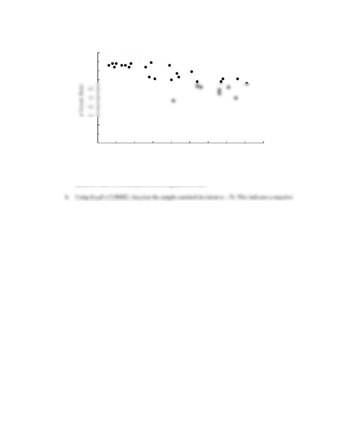
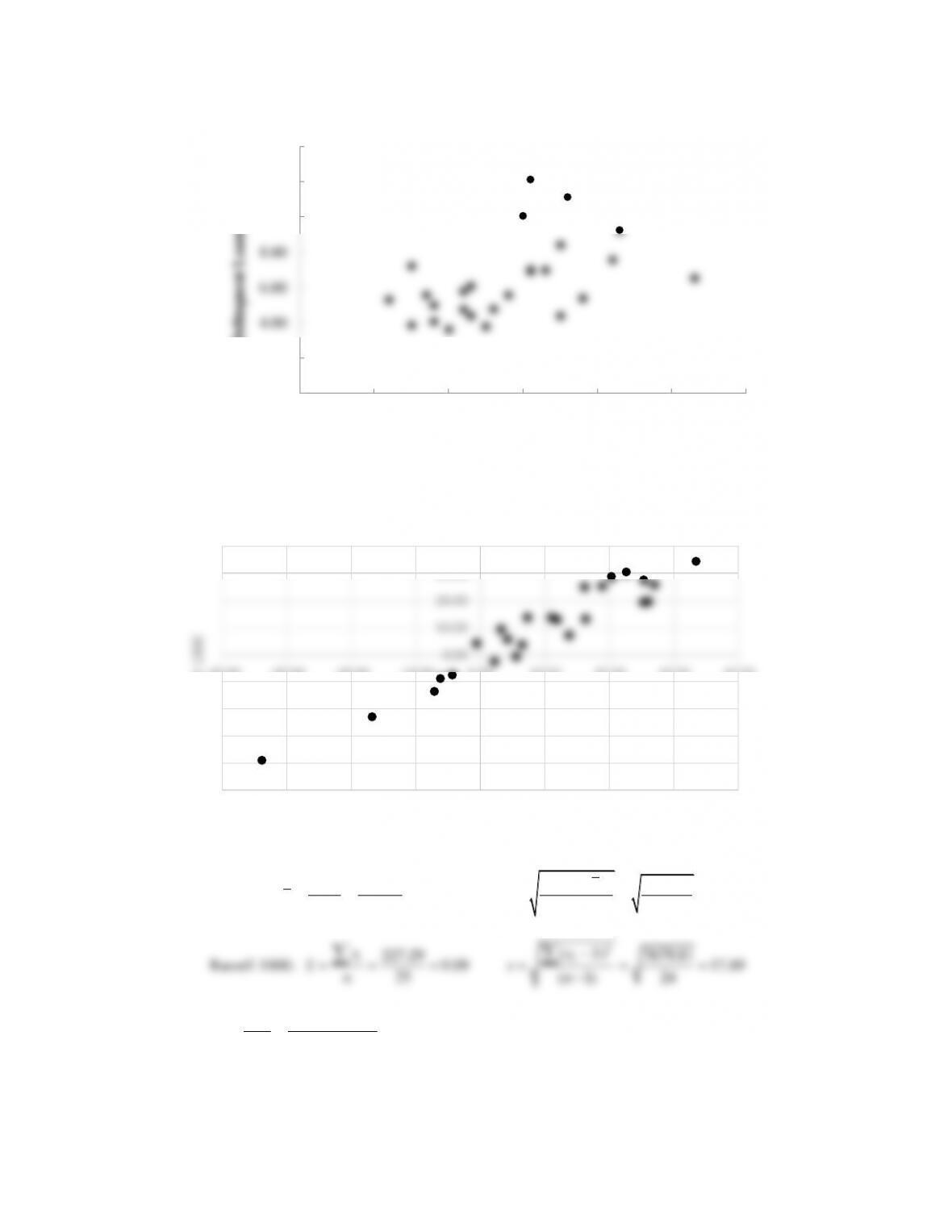
61. a.
There appears to be a negative linear relationship between the two variables. In other words, higher
admission rates are associated with lower graduation rates.
linear relationship between the two variables.
0
10
20
30
40
50
60
70
80
90
100
010 20 30 40 50 60 70 80 90
4-yr Grad. Rate (%)
Admit Rate (%)