40. a.
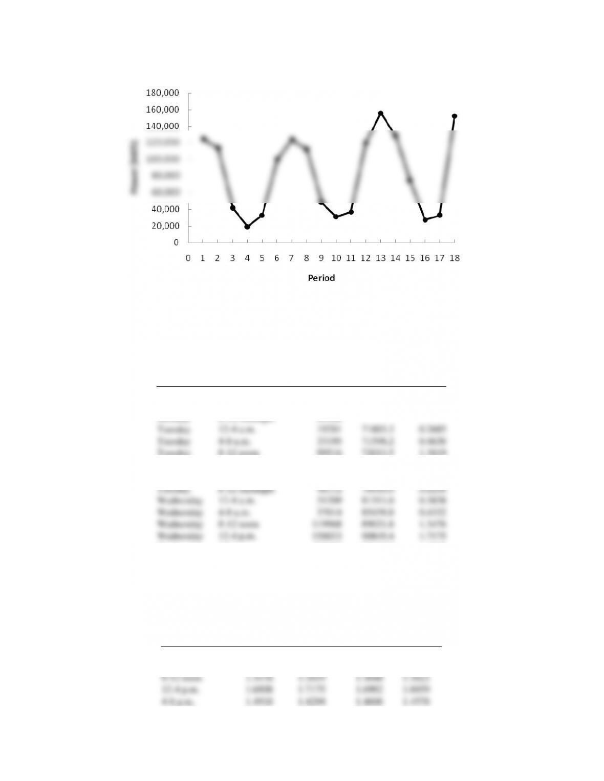
The time series plot indicates a seasonal effect. Power consumption is lowest in the time period 12–4
A.M., steadily increases to the highest value in the 12-4 P.M. time period, and then decreases again.
There may also be some linear trend in the data.
b.
Day
Time Period
Power
Centered
Moving
Average
Seasonal-
Irregular
Values
Monday
12-4 p.m.
124299
Monday
4-8 p.m.
113545
Monday
8-12 midnight
41300
Tuesday
12-4 a.m.
19281
71803.3
0.2685
Tuesday
4-8 a.m.
33195
71598.2
0.4636
Tuesday
8-12 noon
99516
72013.5
1.3819
Tuesday
12-4 p.m.
123666
73575.2
1.6808
Tuesday
4-8 p.m.
111717
74887.4
1.4918
Tuesday
8-12 midnight
48112
76910.0
0.6256
Wednesday
12-4 a.m.
31209
81311.6
0.3838
Wednesday
4-8 a.m.
37014
85439.8
0.4332
Wednesday
8-12 noon
119968
89021.8
1.3476
Wednesday
12-4 p.m.
156033
90849.4
1.7175
Wednesday
4-8 p.m.
128889
90167.9
1.4294
Wednesday
8-12 midnight
73923
92517.8
0.7990
Thursday
12-4 a.m.
27330
Thursday
4-8 a.m.
32715
Thursday
8-12 noon
152465
Time Period
Seasonal-Irregular
Values
Seasonal
Index
Adjusted
Seasonal
Index
12-4 a.m.
0.3838
0.2685
0.3262
0.3256
4-8 a.m.
0.4332
0.4636
0.4484
0.4476
8-12 noon
1.3476
1.3819
1.3648
1.3622
12-4 p.m.
1.6808
1.7175
1.6992
1.6959
4-8 p.m.
1.4918
1.4294
1.4606
1.4578
8-12 midnight
0.6256
0.7990
0.7123
0.7109
Total
6.0114
c.
Day
Time Period
Power
Adjusted
Seasonal
Index
Deseasonalized Power
Monday
12-4 p.m.
124299
1.6959
73292.80
Monday
4-8 p.m.
113545
1.4578
77885.67
Monday
8-12 midnight
41300
0.7109
58092.48
Tuesday
12-4 a.m.
19281
0.3256
59225.36
Tuesday
4-8 a.m.
33195
0.4476
74166.93
Tuesday
8-12 noon
99516
1.3622
73056.72
Tuesday
12-4 p.m.
123666
1.6959
72919.55
Tuesday
4-8 p.m.
111717
1.4578
76631.76
Tuesday
8-12 midnight
48112
0.7109
67674.22
Wednesday
12-4 a.m.
31209
0.3256
95864.54
Wednesday
4-8 a.m.
37014
0.4476
82699.65
Wednesday
8-12 noon
119968
1.3622
88070.95
Wednesday
12-4 p.m.
156033
1.6959
92004.73
Wednesday
4-8 p.m.
128889
1.4578
88410.82
Wednesday
8-12 midnight
73923
0.7109
103979.91
Thursday
12-4 a.m.
27330
0.3256
83949.43
Thursday
4-8 a.m.
32715
0.4476
73094.48
Thursday
8-12 noon
152465
1.3622
111927.66
Using Excel’s Regression tool to fit a linear trend equation to the deseasonalized time series
provides the following estimated regression equation:
Deseasonalized Power = 63108 + 1854t
Deseasonalized Power = 63108 + 1854(19) = 98,334
Seasonal Index for this period = 1.6959
Forecast for 12-4 P.M. = 1.6959(98,334) = 166,764.63 or approximately 166,765 kWh
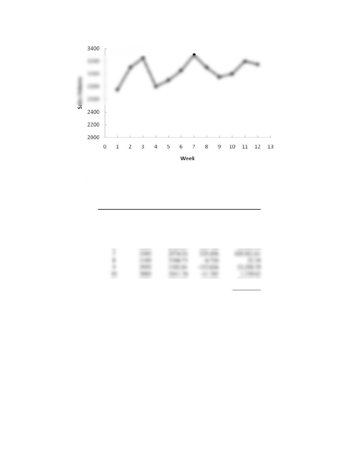
41. a.
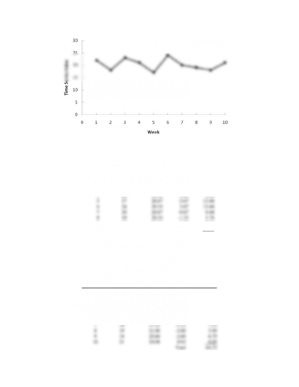
The time series plot indicates a horizontal pattern.
b. Three-week moving average.
Week
Time Series
Value
Forecast
Forecast
Error
Squared
Forecast
Error
1
22
2
18
3
23
4
21
21.00
0.00
0.00
5
17
20.67
-3.67
13.44
6
24
20.33
3.67
13.44
7
20
20.67
-0.67
0.44
8
19
20.33
-1.33
1.78
9
18
21.00
-3.00
9.00
10
21
19.00
2.00
4.00
Total
42.11
MSE = 42.11 / 7 = 6.02
F11 = (19 + 18 + 21) / 3 = 19.33
c. Exponential smoothing using α = .2
Week
Time Series
Value
Forecast
Forecast
Error
Squared Value
of Forecast
Error
1
22
2
18
22.00
-4.00
16.00
3
23
21.20
1.80
3.24
4
21
21.56
-0.56
0.31
5
17
21.45
-4.45
19.78
6
24
20.56
3.44
11.84
7
20
21.25
-1.25
1.55
8
19
21.00
-2.00
3.99
9
18
20.60
-2.60
6.75
10
21
20.08
0.92
0.85
Total
64.33
d. The 3-month moving average is preferable. It has a smaller MSE.
42. a.
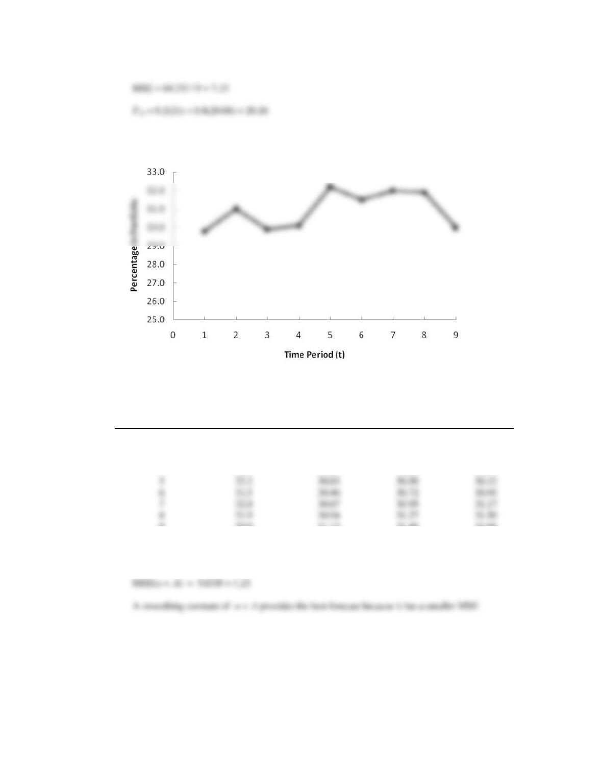
The time series plot indicates a horizontal pattern.
b.
Period
Time Series
Value
α = .2
Forecasts
α = .3
Forecasts
α = .4
Forecasts
1
29.8
2
31.0
29.80
29.80
29.80
3
29.9
30.04
30.16
30.28
4
30.1
30.01
30.08
30.13
5
32.2
30.03
30.09
30.12
6
31.5
30.46
30.72
30.95
7
32.0
30.67
30.95
31.17
8
31.9
30.94
31.27
31.50
9
30.0
31.13
31.46
31.66
MSE(α = .2) = 11.22/8 = 1.40
MSE(α = .3) = 10.19/8 = 1.27
c. Using α = .4, F10 = .4(30) + .6(31.66) = 31.00
43. a.
The time series plot indicates a horizontal pattern.
b.
Week
Sales
Volume
Forecast
Forecast
Error
Squared Value
of Forecast
Error
1
2750
2
3100
2750.00
350.000
122,500.00
3
3250
2890.00
360.000
129,600.00
4
2800
3034.00
-234.000
54,756.00
5
2900
2940.40
-40.400
1,632.16
6
3050
2924.24
125.760
15,815.58
7
3300
2974.54
325.456
105,921.61
8
3100
3104.73
-4.726
22.34
9
2950
3102.84
-152.836
23,358.79
10
3000
3041.70
-41.702
1,739.02
11
3200
3025.02
174.979
30,617.68
12
3150
3095.01
54.987
3,023.62
Total
488,986.80
Note: MSE = 488,986.80/11 = 44,453
Forecast for week 13 = .4(3150) + .6(3095.01) = 3117.01 or 3117 half-gallons of milk.
44. a.
There appears to be an increasing trend in the data through April 2011 followed by periods of
decreasing and increasing cost.
b. Using Excel’s Regression tool, the estimated regression equation is:
c. Using Excel’s Regression tool, the estimated multiple regression equation is:
Cost = 68.82 + 2.08t – .03t2
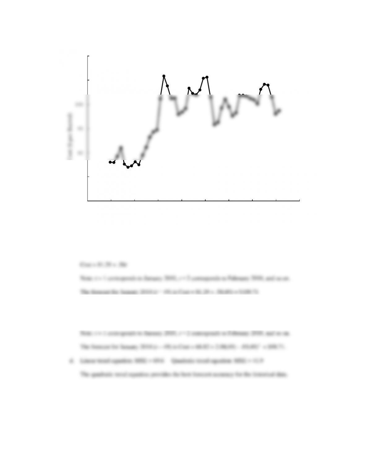
45. a.
60
70
80
90
100
110
120
Jul-2009 Jan-2010 Aug-2010 Feb-2011 Sep-2011 Apr-2012 Oct-2012 May-2013 Nov-2013 Jun-2014
Cost ($ per Barrel)
Date
The time series plot shows a linear trend.
b.
Smoothing Constant
MSE
= .3
4,492.37
= .4
2,964.67
= .5
2,160.31
The
= .5 smoothing constant is better because it has the smallest MSE.
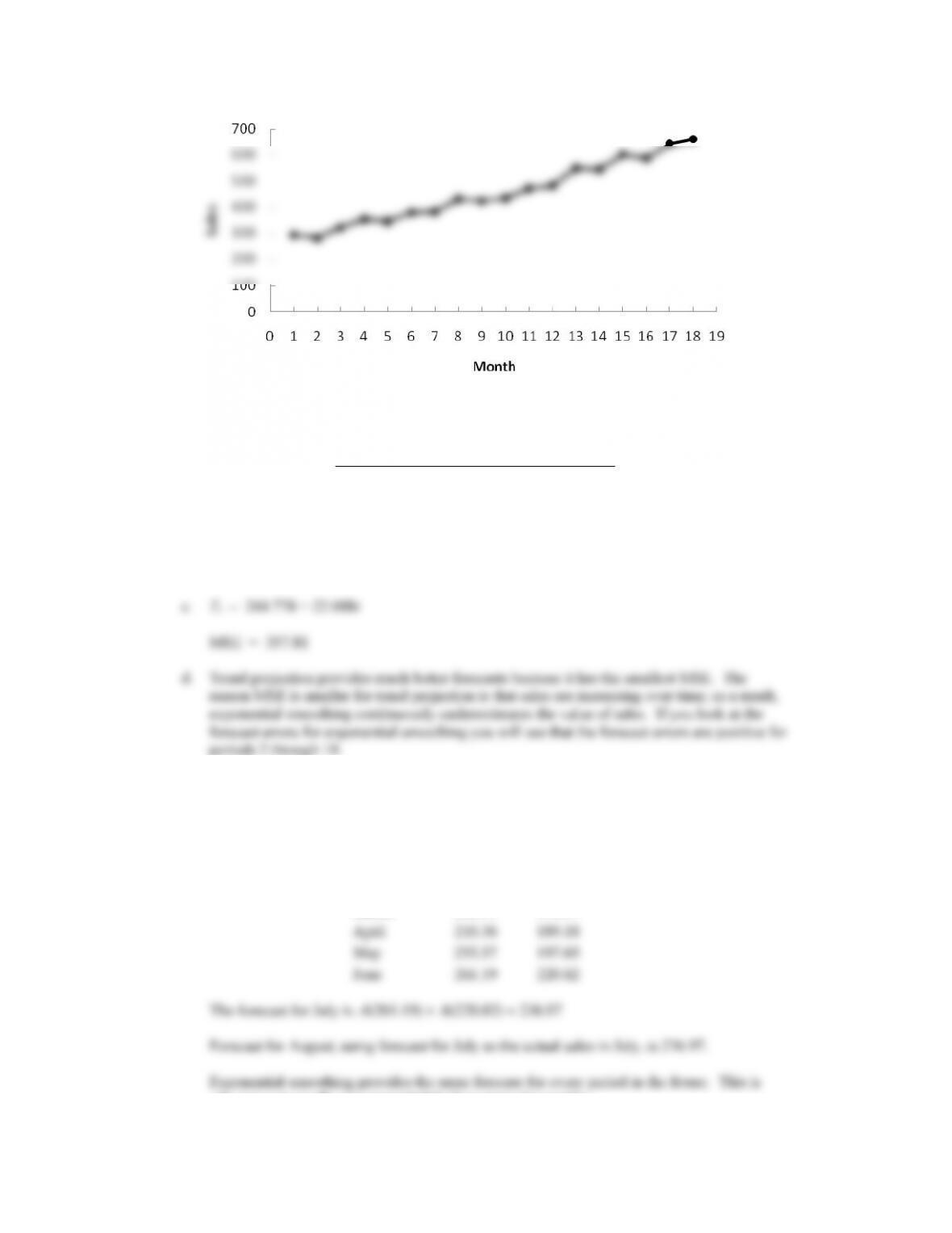
46. a. The following table shows the calculations using a smoothing constant of .4.
Month
Sales
($1000s)
Forecast
January
185.72
February
167.84
185.72
March
205.11
178.57
April
210.36
189.18
May
255.57
197.65
June
261.19
220.82
why it is not usually recommended for long-term forecasting.
b. Using Excel’s Regression tool, the linear trend equation is:
Tt = 149.72 + 18.451t
$278,880 in July and $297,330 in August.
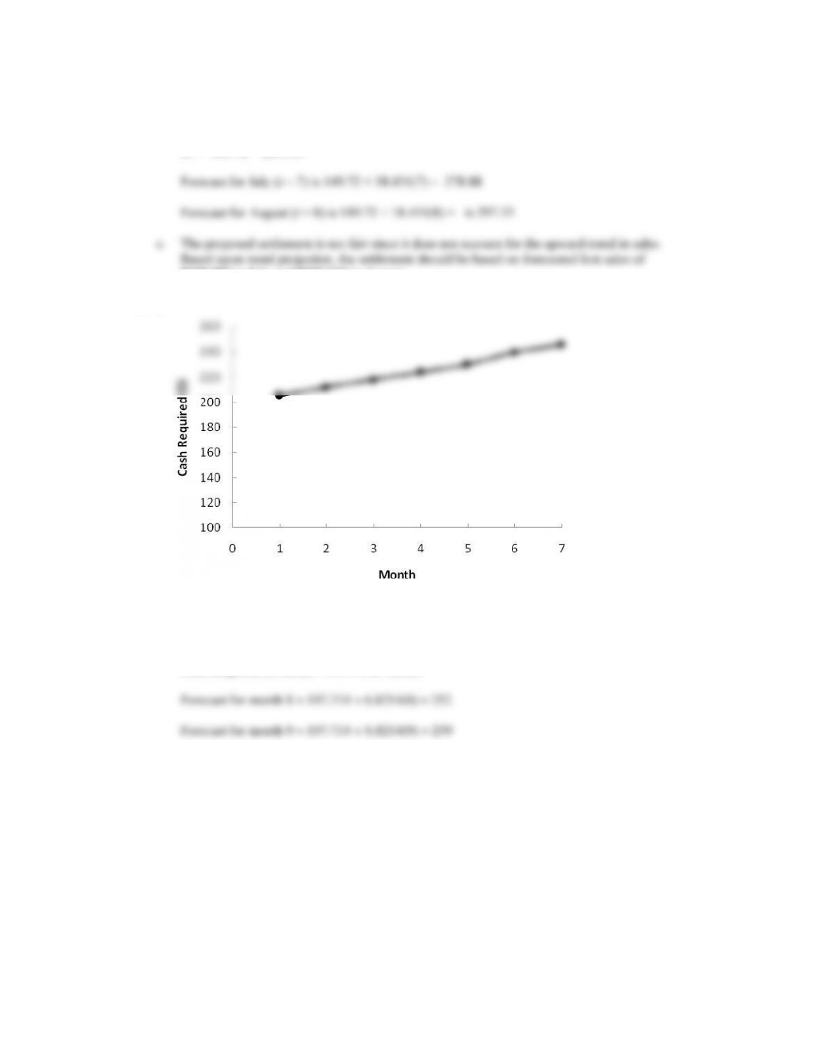
47. a.
The time series plot indicates a linear trend.
b. Using Excel’s Regression tool, the estimated regression equation is:
Cash Required ($1000s) = 198 + 6.82 Month