Unlock document.
This document is partially blurred.
Unlock all pages and 1 million more documents.
Get Access
27. a.
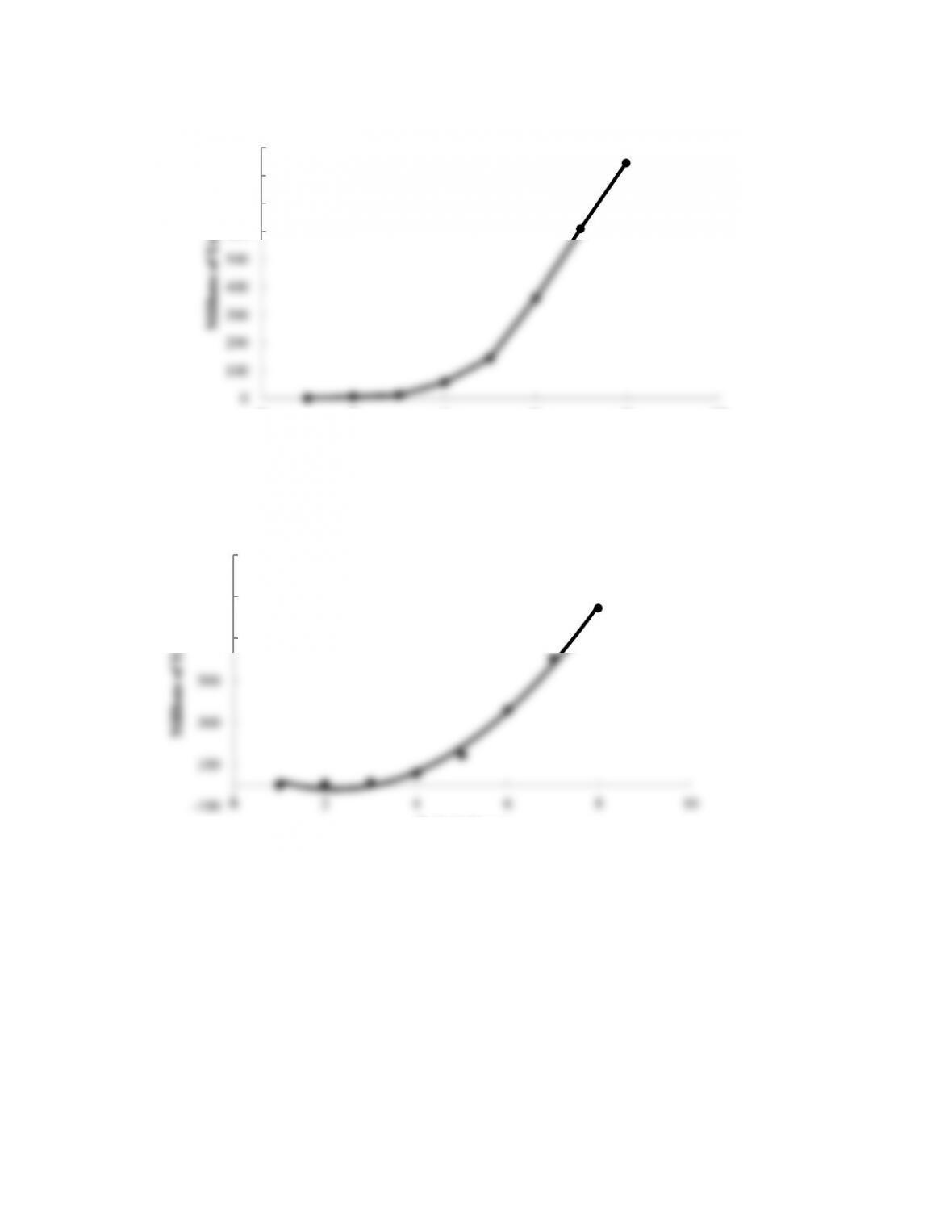
The time series plot indicates curvature in the data.
b. The following output shows the results of using Excel’s Chart tools to fit a quadratic trend equation
to the time series.
28. a.
0
100
200
300
400
500
600
700
800
900
0 2 4 6 8 10
Millions of Users
Period (Year)
y = 26.22x2- 116.35x + 109.34
-100
100
300
500
700
900
1100
0 2 4 6 8 10
Millions of Users
Period (Year)
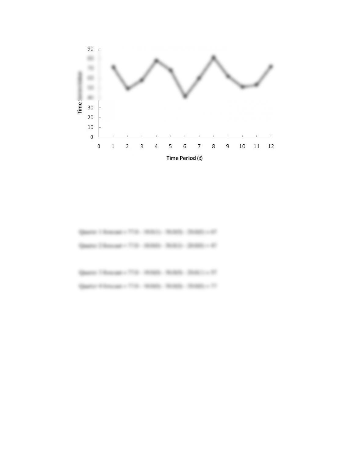
The time series plot shows a horizontal pattern. But, there is a seasonal pattern in the data. For
instance, in each year the lowest value occurs in quarter 2 and the highest value occurs in quarter 4.
b. Using Excel’s Regression tool, the estimated multiple regression equation is:
Value = 77.0 - 10.0 Qtr1 - 30.0 Qtr2 - 20.0 Qtr3
c. The quarterly forecasts for next year are as follows:
29. a.
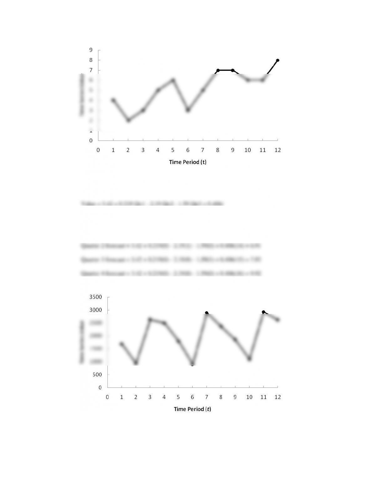
The time series plot shows a linear trend and a seasonal pattern in the data.
b. Using Excel’s Regression tool, the estimated multiple regression equation is:
c. The quarterly forecasts for next year (t = 13, 14, 15, and 16) are as follows:
Quarter 1 forecast = 3.42 + 0.219(1) - 2.19(0) - 1.59(0) + 0.406(13) = 8.92
30. a.
There appears to be a seasonal pattern in the data and perhaps a moderate upward linear trend.
b. Using Excel’s Regression tool, the estimated multiple regression equation is:
Value = 2492 - 712 Qtr1 - 1512 Qtr2 + 327 Qtr3
c. The quarterly forecasts for next year are as follows:
Quarter 1 forecast = 2492 – 712(1) – 1512(0) + 327(0) = 1780
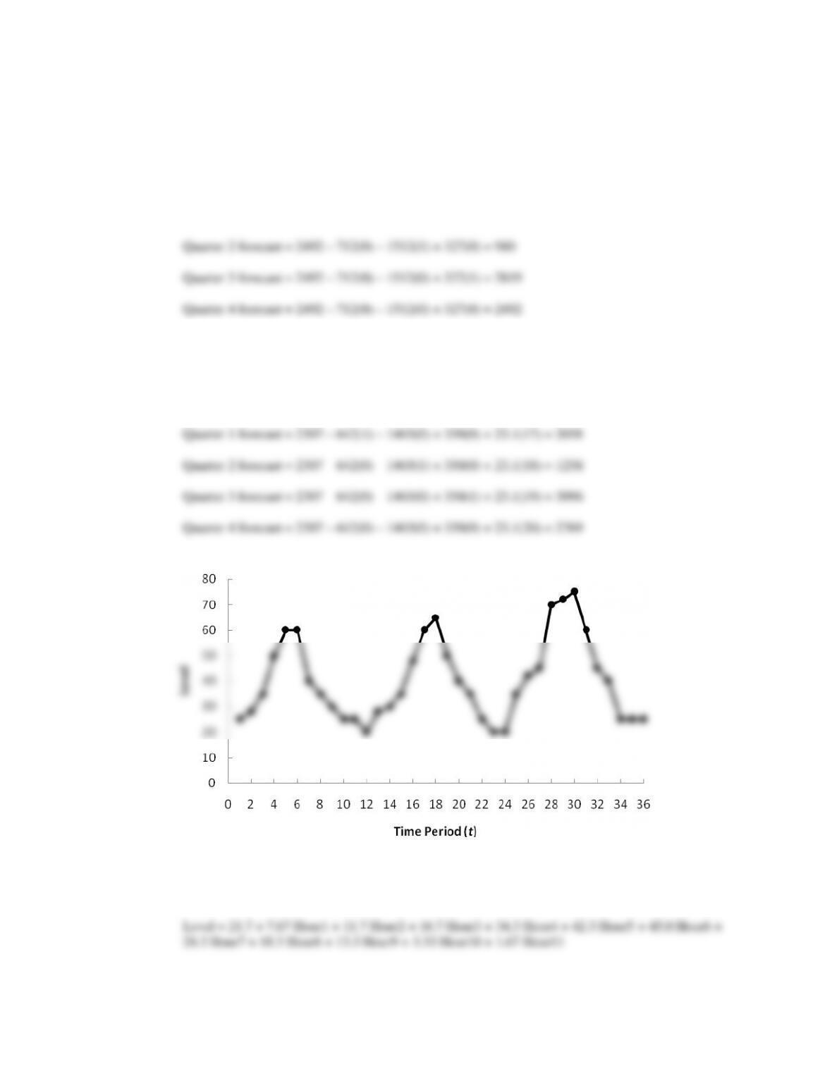
d. Using Excel’s Regression tool, the estimated multiple regression equation is:
Value = 2307 - 642 Qtr1 - 1465 Qtr2 + 350 Qtr3 + 23.1t
The quarterly forecasts for next year are as follows:
31. a.
The time series plot indicates a seasonal pattern in the data and perhaps a slight upward linear trend.
b. Using Excel’s Regression tool, the estimated multiple regression equation is:
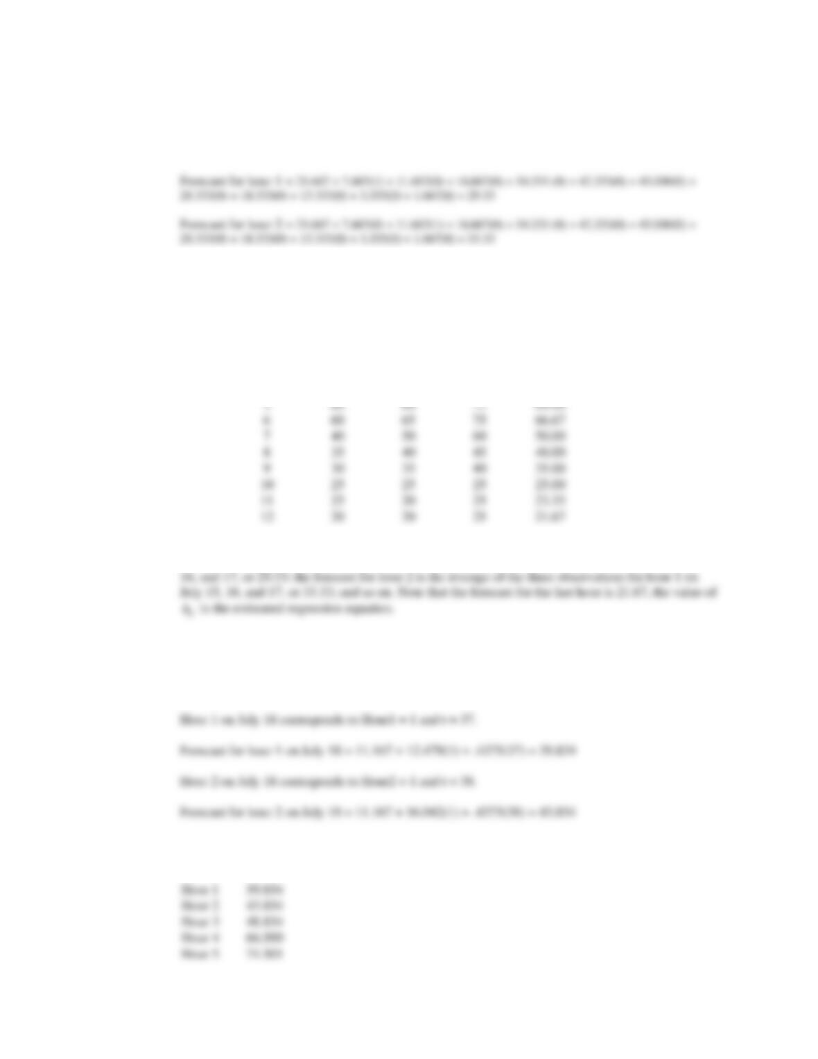
c. The hourly forecasts for the next day can be obtained very easily using the estimated regression
equation. For instance, setting Hour1 = 1 and the rest of the dummy variables equal to 0 provides the
forecast for the first hour; setting Hour2 = 1 and the rest of the dummy variables equal to 0 provides
the forecast for the second hour; and so on.
The forecasts for the remaining hours can be obtained similarly. But, since there is no trend the data the hourly
forecasts can also be computed by simply taking the average of the three time series values for each hour.
Hour
July 15
July 16
July 17
Average
1
25
28
35
29.33
2
28
30
42
33.33
3
35
35
45
38.33
4
50
48
70
56.00
5
60
60
72
64.00
6
60
65
75
66.67
7
40
50
60
50.00
8
35
40
45
40.00
9
30
35
40
35.00
10
25
25
25
25.00
11
25
20
25
23.33
12
20
20
25
21.67
In other words, the forecast for hour 1 is the average of the three observations for hour 1 on July 15,
0
d. Using Excel’s Regression tool, the estimated multiple regression equation is:
Level = 11.2 + 12.5 Hour1 + 16.0 Hour2 + 20.6 Hour3 + 37.8 Hour4 + 45.4 Hour5 + 47.6 Hour6 +
30.5 Hour7 + 20.1 Hour8 + 14.6 Hour9 + 4.21 Hour10 + 2.10 Hour11 + 0.437t
The forecasts for the other hours are computed in a similar manner. The following table shows the
forecasts for the 12 hours on July 18.
Hour 1
39.834
Hour 2
43.834
Hour 3
48.834
Hour 4
66.500
Hour 5
74.501
Hour 6
77.167
Hour 7
60.501
Hour 8
50.500
Hour 9
45.501
Hour 10
35.500
Hour 11
33.834
Hour 12
32.167
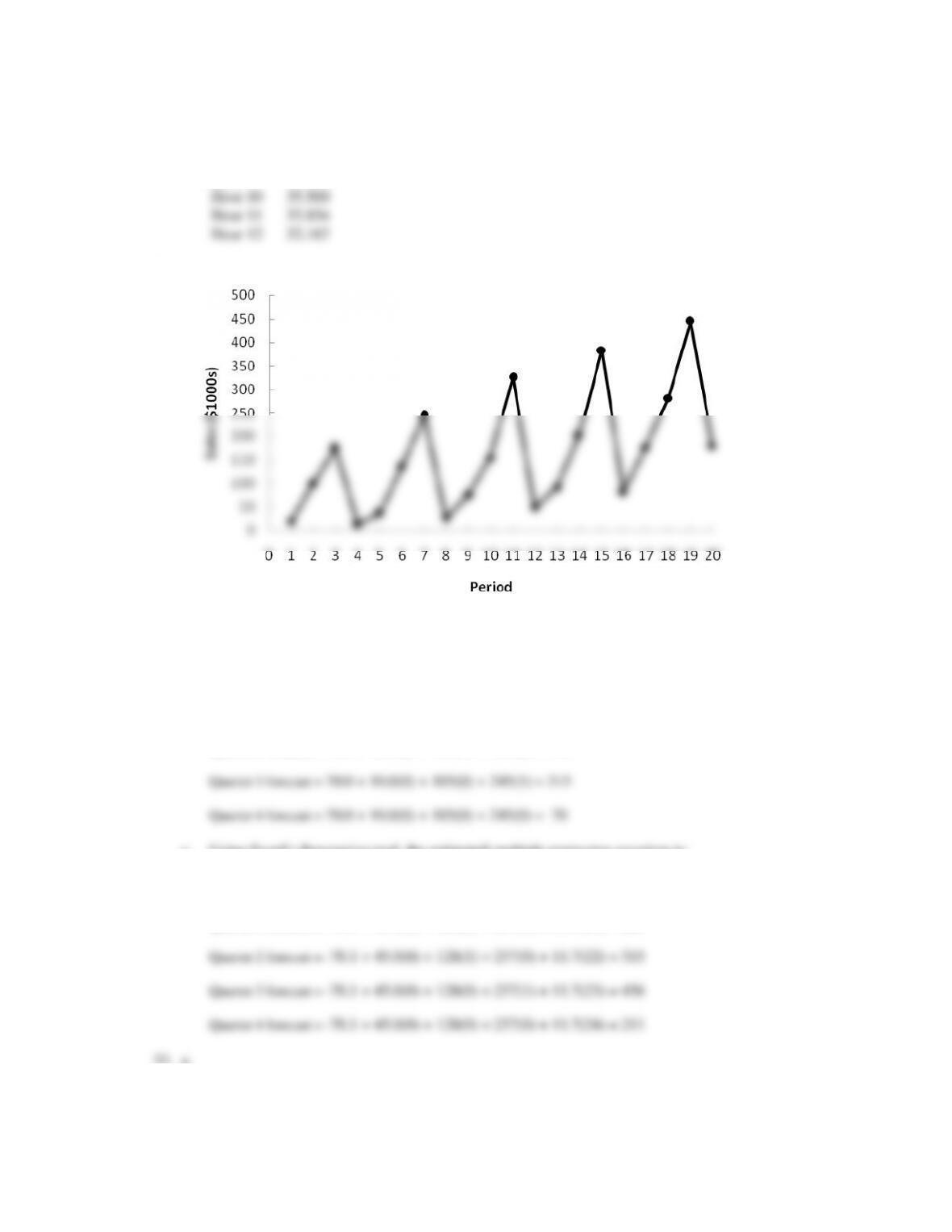
32. a.
The time series plot shows both a linear trend and seasonal effects.
b. Using Excel’s Regression tool, the estimated regression equation is:
Revenue = 70.0 + 10.0 Qtr1 + 105 Qtr2 + 245 Qtr3
Quarter 1 forecast = 70.0 + 10.0(1) + 105(0) + 245(0) = 80
Quarter 2 forecast = 70.0 + 10.0(0) + 105(1) + 245(0) = 175
c. Using Excel’s Regression tool, the estimated multiple regression equation is:
Revenue = - 70.1 + 45.0 Qtr1 + 128 Qtr2 + 257 Qtr3 + 11.7 Period
Quarter 1 forecast = -70.1 + 45.0(1) + 128(0) + 257(0) + 11.7(21) = 221
33. a.
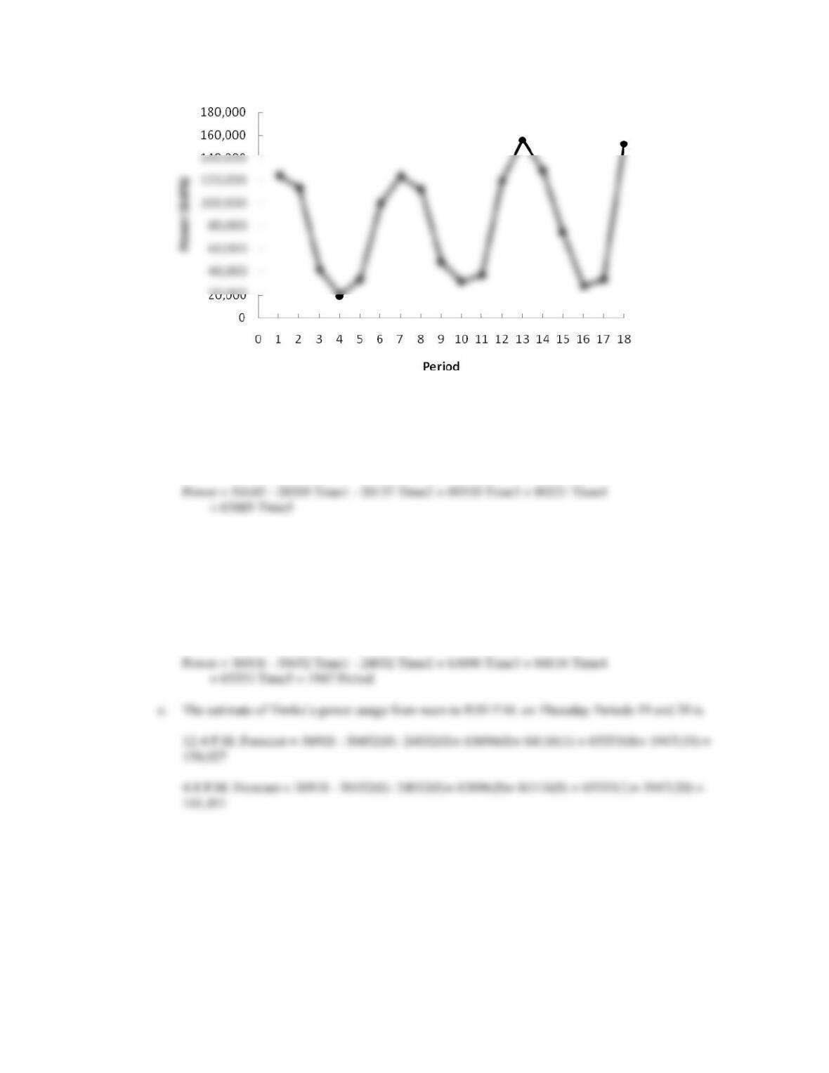
The time series plot indicates a seasonal effect. Power consumption is lowest in the time period 12-4
A.M., steadily increases to the highest value in the 12-4 P.M. time period, and then decreases again.
There may also be some linear trend in the data.
b. Using Excel’s Regression tool, the estimated multiple regression equation is:
c. The estimate of Timko’s power usage from noon to 8:00 P.M. on Thursday is
12-4 P.M. Forecast = 54445 – 28505(0) - 20137(0)+ 69538(0)+ 80221(1)+ 63605(0) = 134,666
4-8 P.M. Forecast = 54445 – 28505(0) - 20137(0)+ 69538(0)+ 80221(0)+ 63605(1) = 118,050
d. Using Excel’s Regression tool, the estimated multiple regression equation is:
Power = 36918 - 30452 Time1 - 24032 Time2 + 63696 Time3 + 84116 Time4
34. a.
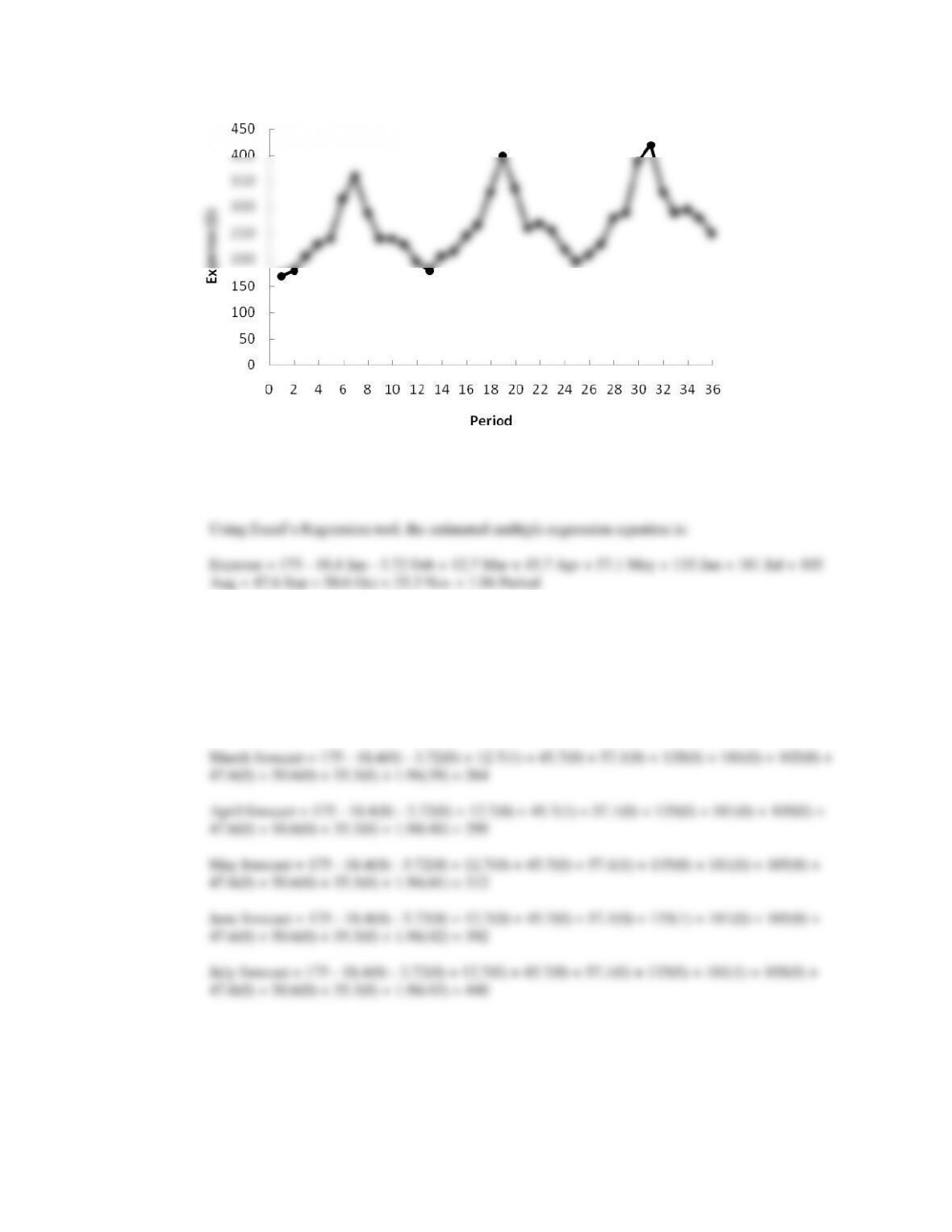
The time series plot shows seasonal and linear trend effects.
b. Note: Jan = 1 if January, 0 otherwise; Feb = 1 if February, 0 otherwise; and so on.
c. Note: The next time period in the time series is Period = 37 (January of Year 4).
January forecast = 175 - 18.4(1) - 3.72(0) + 12.7(0) + 45.7(0) + 57.1(0) + 135(0) + 181(0) + 105(0)
+ 47.6(0) + 50.6(0) + 35.3(0) + 1.96(37) = 229
February forecast = 175 - 18.4(0) - 3.72(1) + 12.7(0) + 45.7(0) + 57.1(0) + 135(0) + 181(0) + 105(0)
+ 47.6(0) + 50.6(0) + 35.3(0) + 1.96(38) = 246
August forecast = 175 - 18.4(0) - 3.72(0) + 12.7(0) + 45.7(0) + 57.1(0) + 135(0) + 181(0) + 105(1) +
47.6(0) + 50.6(0) + 35.3(0) + 1.96(44) = 366
September forecast = 175 - 18.4(0) - 3.72(0) + 12.7(0) + 45.7(0) + 57.1(0) + 135(0) + 181(0) +
105(0) + 47.6(1) + 50.6(0) + 35.3(0) + 1.96(45) = 311
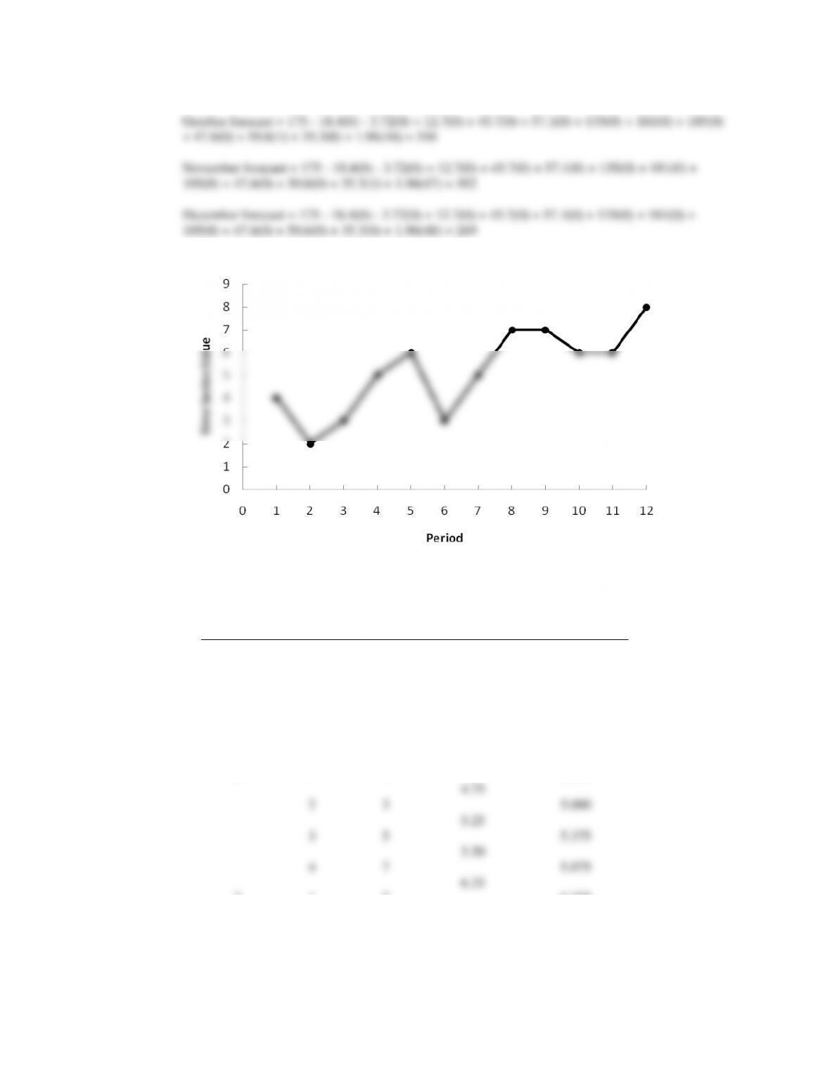
35. a.
The time series plot indicates a linear trend and a seasonal pattern.
b.
Year
Quarter
Time Series
Value
Four-Quarter
Moving Average
Centered Moving
Average
1
1
4
2
2
3.50
3
3
3.750
4.00
4
5
4.125
4.25
2
1
6
4.500
4.75
2
3
5.000
5.25
3
5
5.375
5.50
4
7
5.875
6.25
3
1
7
6.375
6.50
2
6
6.625
6.75
3
6
4
8
c.
Year
Quarter
Time Series
Value
Centered Moving
Average
Seasonal-
Irregular Value
1
1
4
2
2
3
3
3.750
0.800
4
5
4.125
1.212
2
1
6
4.500
1.333
2
3
5.000
0.600
3
5
5.375
0.930
4
7
5.875
1.191
3
1
7
6.375
1.098
2
6
6.625
0.906
3
6
4
8
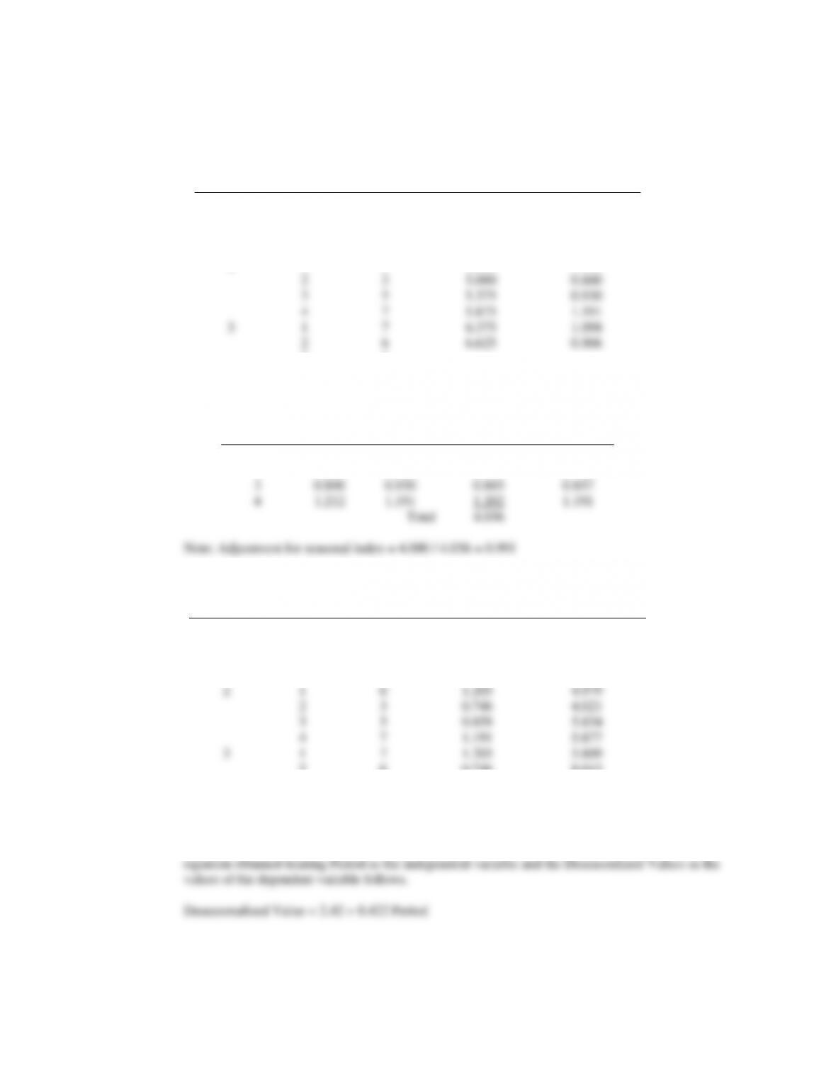
Quarter
Seasonal-Irregular
Values
Seasonal Index
Adjusted
Seasonal
Index
1
1.333
1.098
1.216
1.205
2
0.600
0.906
0.753
0.746
3
0.800
0.930
0.865
0.857
4
1.212
1.191
1.202
1.191
Total
4.036
36. a.
Year
Quarter
Time Series
Value
Adjusted
Seasonal Index
Deseasonalized
Value
1
1
4
1.205
3.320
2
2
0.746
2.681
3
3
0.858
3.501
4
5
1.191
4.198
2
1
6
1.205
4.979
2
3
0.746
4.021
3
5
0.858
5.834
4
7
1.191
5.877
3
1
7
1.205
5.809
2
6
0.746
8.043
3
6
0.858
7.001
4
8
1.191
6.717
b. Let Period = 1 denote the time series value in Year 1 – Quarter 1; Period = 2 denote the time series
value in Year 1 – Quarter 2; and so on. Using Excel’s Regression tool, the estimated regression
c. The quarterly deseasonalized trend forecasts for Year 4 (Periods 13, 14, 15, and 16) are as follows:
Forecast for quarter 1 = 2.42 + 0.422(13) = 7.906

Forecast for quarter 2 = 2.42 + 0.422(14) = 8.328
d. Adjusting the quarterly deseasonalized trend forecasts provides the following quarterly estimates:
Forecast for quarter 1 = 7.906(1.205) = 9.527
Forecast for quarter 2 = 8.328(.746) = 6.213


