32. a. E(y) =
+
x1 +
x2 where
x2 = 0 if level 1 and 1 if level 2
33. a. two
b. E(y) =
+
x1 +
x2 +
x3 where
x2
x3
Level
0
0
1
1
0
2
0
1
3
is the change in E(y) for a 1 unit change in x1 holding x2 and x3 constant.
34. a. $15,300
c. Estimate of sales = 10.1 – 4.2(1) + 6.8(3) + 15.3(1) = 41.6 or $41,600
35. a. Let Type = 0 if a mechanical repair
Type = 1 if an electrical repair
The Excel output is shown below:
Regression Statistics
Multiple R
0.2952
R Square
0.0871
Adjusted R Square
-0.0270
Standard Error
1.0934
Observations
10
ANOVA
df
SS
MS
F
Significance F
Regression
1
0.9127
0.9127
0.7635
0.4077
Residual
8
9.5633
1.1954
Total
9
10.476
Coefficients
Standard Error
t Stat
P-value
Intercept
3.45
0.5467
6.3109
0.0002
Type
0.6167
0.7058
0.8738
0.4077
ˆ
y
= 3.45 + .6167 Type
that the relationship is not significant for any reasonable value of
.
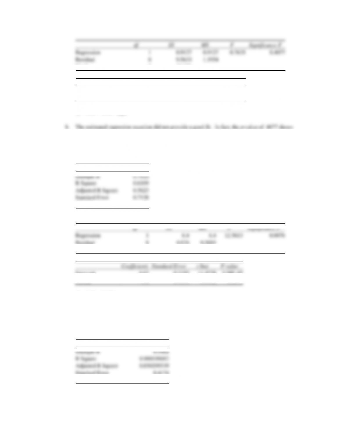
c. Person = 0 if Bob Jones performed the service and Person = 1 if Dave Newton performed the
service. The Excel output is shown below:
Regression Statistics
Multiple R
0.7816
R Square
0.6109
Adjusted R Square
0.5623
Standard Error
0.7138
Observations
10
ANOVA
df
SS
MS
F
Significance F
Regression
1
6.4
6.4
12.5613
0.0076
Residual
8
4.076
0.5095
Total
9
10.476
Coefficients
Standard Error
t Stat
P-value
Intercept
4.62
0.3192
14.4729
5.08E-07
Person
-1.6
0.4514
-3.5442
0.0076
ˆ
y
= 4.62 – 1.6 Person
d. We see that 61.1% of the variability in repair time has been explained by the repair person that
performed the service; an acceptable, but not good, fit.
36. a. The Excel output is shown below:
Regression Statistics
Multiple R
0.9488
R Square
0.900199692
Adjusted R Square
0.850299539
Standard Error
0.4174
Observations
10
ANOVA
df
SS
MS
F
Significance F
Regression
3
9.4305
3.1435
18.0400
0.0021
Residual
6
1.0455
0.1743
Total
9
10.476
Coefficients
Standard Error
t Stat
P-value
Intercept
1.8602
0.7286
2.5529
0.0433
Months Since Last Service
0.2914
0.0836
3.4862
0.0130
Type
1.1024
0.3033
3.6342
0.0109
Person
-0.6091
0.3879
-1.5701
0.1674
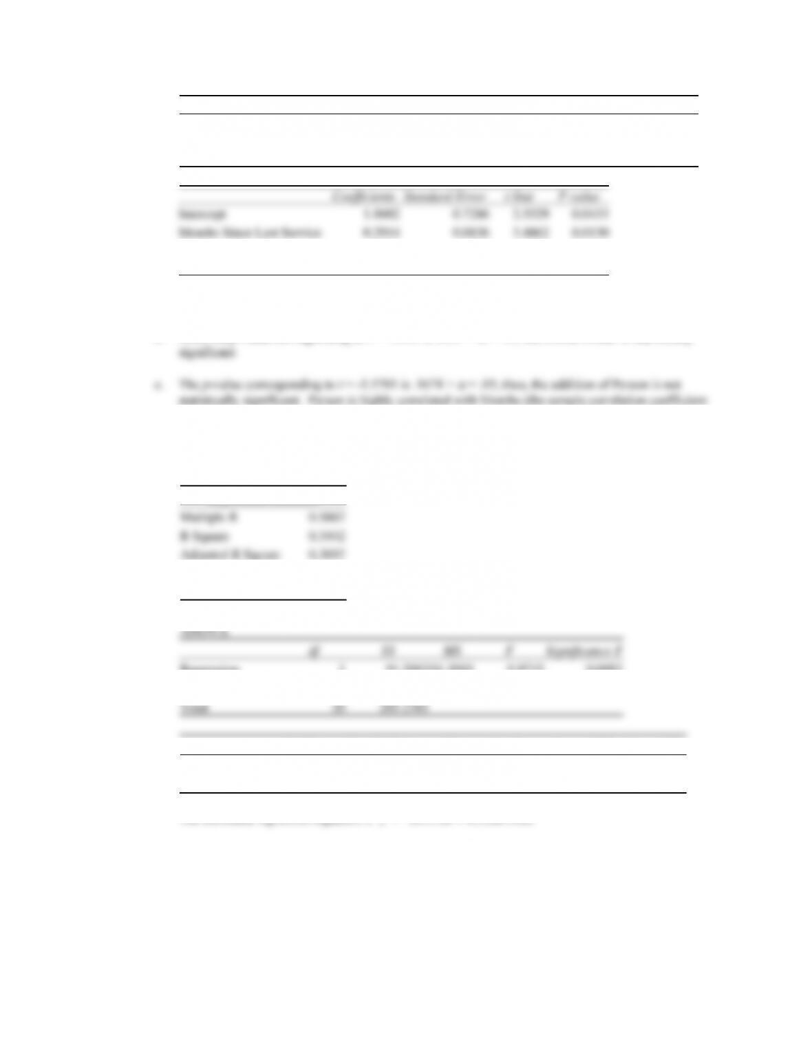
ˆ
y
= 1.8602 + .2914 Months + 1.1024 Type – .6091 Person
b. Since the p-value corresponding to F = 18.04 is .0021 <
= .05, the overall model is statistically
is -.691); thus, once the effect of Months has been accounted for, Person will not add much to the
model.
37. a. A portion of the Excel output follows:
Regression Statistics
Multiple R
0.5867
R Square
0.3442
Adjusted R Square
0.3097
Standard Error
3.0257
Observations
21
ANOVA
df
SS
MS
F
Significance F
Regression
1
91.2902
91.2902
9.9715
0.0052
Residual
19
173.9479
9.1552
Total
20
265.2381
Coefficients
Standard Error
t Stat
P-value
Lower 95%
Upper 95%
Intercept
69.2760
3.4005
20.3725
2.27644E-14
62.1588
76.3933
Price ($)
0.5586
0.1769
3.1578
0.0052
0.1883
0.9288
The estimated regression equation is
ˆ
y
= 69.2760 + 0.5586 Price
b. Because the p-value = .0052 < α = .05, there is a significant relationship.
c. Let Type_Italian = 1 if the restaurant is an Italian restaurant; 0 otherwise
d. A portion of the Excel output follows:
Regression Statistics
Multiple R
0.7254
R Square
0.5262
Adjusted R Square
0.4736
Standard Error
2.6422
Observations
21
ANOVA
df
SS
MS
F
Significance F
Regression
2
139.5771
69.789
9.9967
0.0012
Residual
18
125.6610
6.9812
Total
20
265.2380952
Coefficients
Standard Error
t Stat
P-value
Lower 95%
Upper 95%
Intercept
67.4049
3.0535
22.075
1.74112E-14
60.9898
73.8199
Price ($)
0.5734
0.1546
3.7097
0.0016
0.2487
0.8982
Type_Italian
3.0382
1.1552
2.63
0.0170
0.6112
5.4652
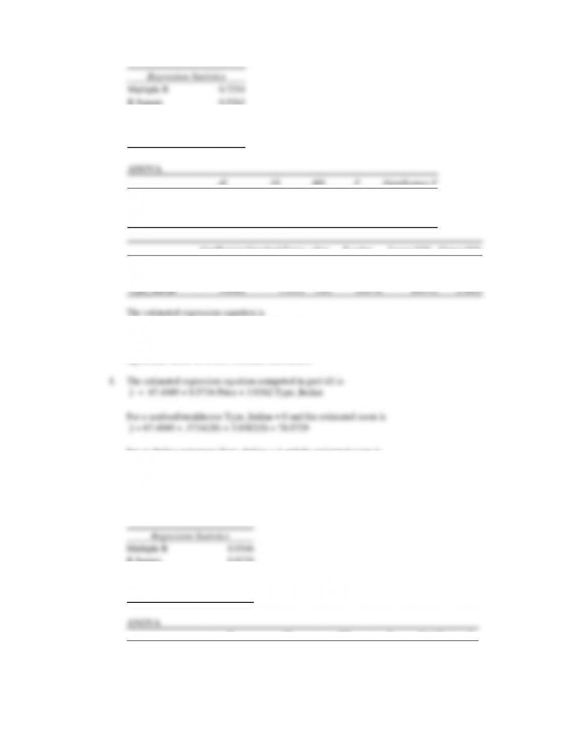
ˆ
y
= 67.4049 + 0.5734 Price + 3.0382 Type_Italian
e. For the Type_Italian dummy variable, the p-value = .0170 < α = .05; thus, type of restaurant is a
significant factor in overall customer satisfaction.
ˆ
y
ˆ
y
For an Italian restaurant Type_Italian = 1 and the estimated score is
ˆ
y
= 67.4049 + .5734(20) + 3.0382(1) = 81.9111
Thus, the satisfaction score increases by 3.0382 points.
38. a. The Excel output is shown below:
R Square
0.8735
Adjusted R Square
0.8498
Standard Error
5.7566
Observations
ANOVA
F
Significance F
Residual
33.1382

Total
19
4190.95
Coefficients
Standard Error
t Stat
P-value
Intercept
-91.7595
15.2228
-6.0278
1.76E-05
Age
1.0767
0.1660
6.4878
7.49E-06
Pressure
0.2518
0.0452
5.5680
4.24E-05
Smoker
8.7399
3.0008
2.9125
0.0102
ˆ
y
= -91.7595 + 1.0767 Age + .2518 Pressure + 8.7399 Smoker
c. The point estimate is 34.27; the 95% prediction interval is 21.35 to 47.18. Thus, the probability of a
stroke (.2135 to .4718 at the 95% confidence level) appears to be quite high. The physician would
probably recommend that Art quit smoking and begin some type of treatment designed to reduce his
blood pressure.
39. a. The Excel output is shown below:
Regression Statistics
Multiple R
0.7946
R Square
0.6314
Adjusted R Square
0.5393
Standard Error
7.2693
Observations
6
ANOVA
df
SS
MS
F
Significance F
Regression
1
362.1304802
362.1305
6.8530
0.0589
Residual
4
211.3695198
52.8424
Total
5
573.5
Coefficients
Standard Error
t Stat
P-value
Intercept
-6.7745
14.1709
-0.4781
0.6576
x
1.2296
0.4697
2.6178
0.0589
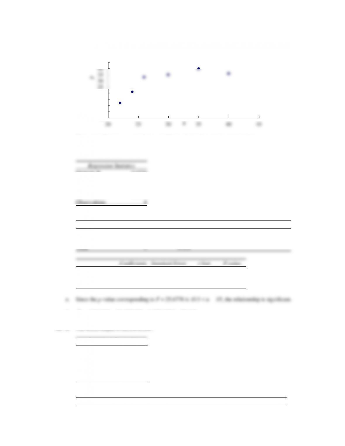
The scatter diagram suggests that a curvilinear relationship may be appropriate.
d. The Excel output is shown below:
Regression Statistics
Multiple R
0.9720
R Square
0.9448
Adjusted R Square
0.9080
Standard Error
3.2482
Observations
6
ANOVA
df
SS
MS
F
Significance F
Regression
2
541.8473
270.9236
25.6778
0.0130
Residual
3
31.6527
10.5509
Total
5
573.5
Coefficients
Standard Error
t Stat
P-value
Intercept
-168.8848
39.7862
-4.2448
0.0239
x
12.1870
2.6632
4.5760
0.0196
xsq
-0.1770
0.0429
-4.1271
0.0258
f.
ˆ
y
= -168.8848 + 12.1870(25) – 0.1770(25)2 = 25.165
40. a. The Excel output is shown below:
Regression Statistics
Multiple R
0.7833
R Square
0.6136
Adjusted R Square
0.4848
Standard Error
3.5311
Observations
5
ANOVA
df
SS
MS
F
Significance F
0
5
10
15
20
25
30
35
40
45
20 25 30 35 40 45
y
x
Regression
1
59.3939
59.3939
4.7634
0.1171
Residual
3
37.4061
12.4687
Total
4
96.8
Coefficients
Standard Error
t Stat
P-value
Intercept
9.3152
4.1961
2.2200
0.1130
x
0.4242
0.1944
2.1825
0.1171
been explained by x.
b. The Excel output is shown below:
Regression Statistics
Multiple R
0.9830
R Square
0.9662
Adjusted R Square
0.9324
Standard Error
1.2788
Observations
5
ANOVA
df
SS
MS
F
Significance F
Regression
2
93.5293
46.7647
28.5963
0.0338
Residual
2
3.2707
1.6353
Total
4
96.8
Coefficients
Standard
Error
t Stat
P-value
Intercept
-8.1014
4.1038
-1.9741
0.1871
x
2.4127
0.4409
5.4724
0.0318
xsq
-0.0480
0.0105
-4.5688
0.0447
At the .05 level of significance, the relationship is significant; the fit is excellent.
41. a. The Excel output is shown below:
Regression Statistics
Multiple R
0.9426
R Square
0.8884
Adjusted R Square
0.8606
Standard Error
32.2940
Observations
6
ANOVA
df
SS
MS
F
Significance F
Regression
1
33223.2143
33223.2143
31.8564
0.0049

Residual
4
4171.6190
1042.9048
Total
5
37394.8333
Coefficients
Standard Error
t Stat
P-value
Intercept
943.0476
59.3802
15.8815
9.18737E-05
x
8.7143
1.5440
5.6441
0.0049
The p-value of .0049 < α = .01; reject H0
Regression Statistics
Multiple R
0.9899
R Square
0.9799
Adjusted R Square
0.9665
Standard Error
15.8264
Observations
6
ANOVA
df
SS
MS
F
Significance F
Regression
2
36643.4048
18321.7024
73.1475
0.0028
Residual
3
751.4286
250.4762
Total
5
37394.8333
Coefficients
Standard Error
t Stat
P-value
Intercept
432.5714
141.1763
3.0641
0.0548
x
37.4286
7.8074
4.7940
0.0173
xsq
-0.3829
0.1036
-3.6952
0.0344
Because the p = value corresponding to F = 73.1475 is .0028 <
= .05, the relationship is significant.
c.
ˆ
y
= 432.5714 +37.4286x – .3829
2
x
= 432.5714 +37.4286(38) – .3829
2
(38)
= 1302
b. No; the relationship appears to be curvilinear.
c.
ˆ
y
= 2.90 – 0.185x + .00351x2
2.91
a
R=
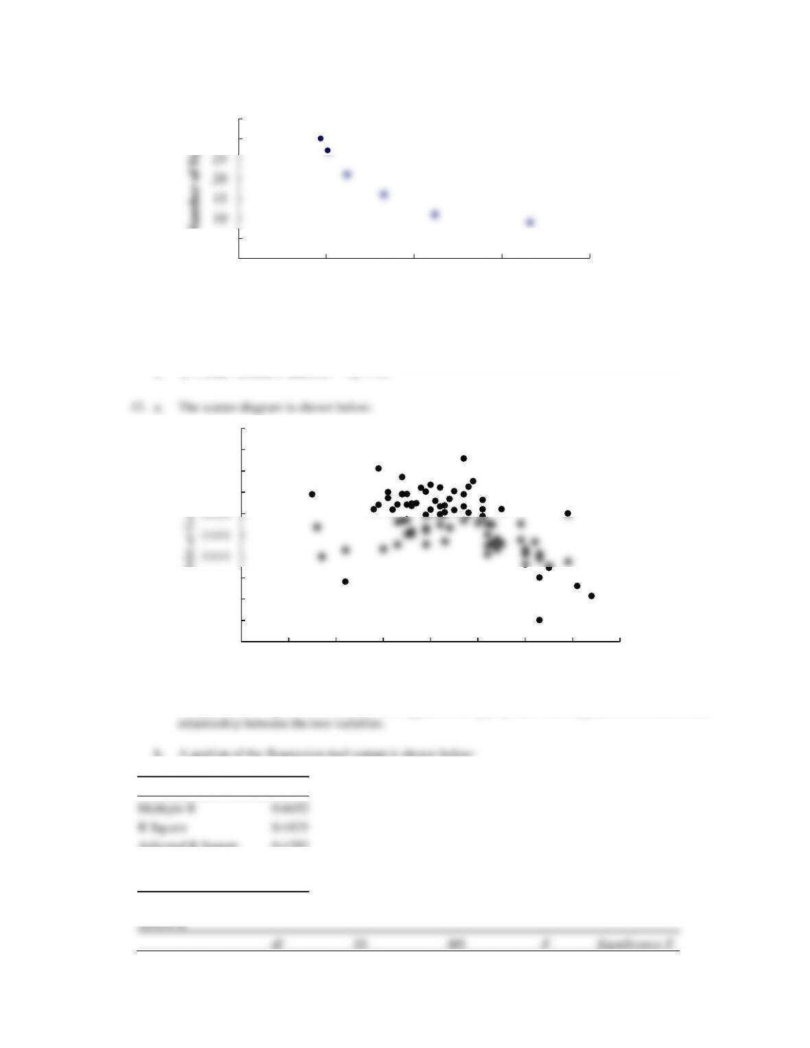
A simple linear regression model does not appear to be appropriate. There appears to be a curvilinear
b. A portion of the Regression tool output is shown below:
Regression Statistics
Multiple R
0.6652
R Square
0.4425
Adjusted R Square
0.4292
Standard Error
5241.4141
Observations
87
ANOVA
df
SS
MS
F
Significance F
0
5
10
15
20
25
30
35
0 0.5 1 1.5 2
y= Number of Facilities
x= Average Distance (miles)
0
5000
10000
15000
20000
25000
30000
35000
40000
45000
50000
010 20 30 40 50 60 70 80
Average Debt at Graduation ($)
% Need-Based Aid

Regression
2
1831419124
915709561.9
33.3320
2.20466E-11
Residual
84
2307683424
27472421.71
Total
86
4139102547
Coefficients
Standard Error
t Stat
P-value
Lower 95%
Upper 95%
Intercept
10092.7919
5396.4997
1.8702
0.0649
-638.7395
20824.323
x
1142.0607
245.4826
4.6523
1.21119E-05
653.8917
1630.2298
xsq
-15.4401
2.6767
-5.7684
1.29806E-07
-20.7629
-10.1172
44. a. The expected increase in final college grade point average corresponding to a one point increase in
high school grade point average is .0235 when SAT mathematics score does not change. Similarly,
the expected increase in final college grade point average corresponding to a one point increase in
the SAT mathematics score is .00486 when the high school grade point average does not change.
b.
ˆ
y
= -1.41 + .0235(84) + .00486(540) = 3.19
45. a. Job satisfaction can be expected to decrease by 8.69 units with a one unit increase in length of
service if the pay grade does not change. A dollar increase in the pay grade is associated with a 13.5
point increase in the job satisfaction score when the length of service does not change.
b.
ˆ
y
= 14.4 – 8.69(4) + 13.5(6) = 60.64