Unlock document.
This document is partially blurred.
Unlock all pages and 1 million more documents.
Get Access
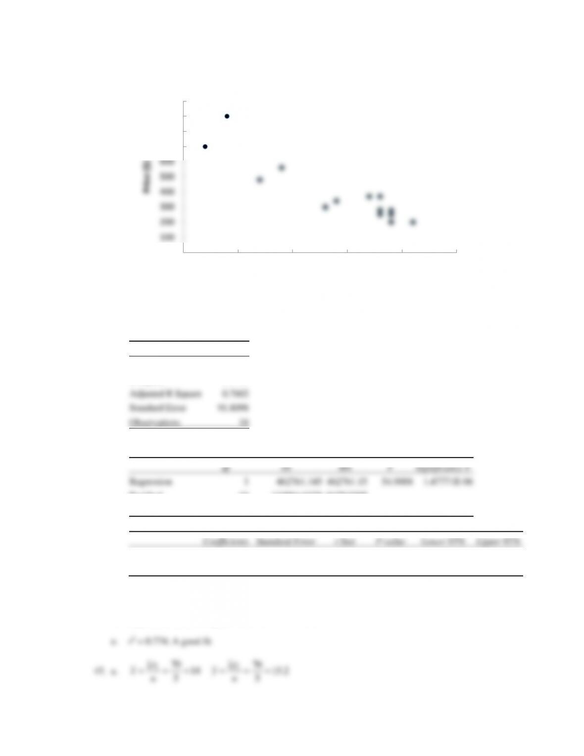
44. a. Scatter diagram:
b. There appears to be a negative linear relationship between the two variables. The heavier helmets
tend to be less expensive.
c. The Excel output is shown below:
Regression Statistics
Multiple R
0.8800
R Square
0.7743
Adjusted R Square
0.7602
Standard Error
91.8098
Observations
18
ANOVA
df
SS
MS
F
Significance F
Regression
1
462761.145
462761.15
54.9008
1.47771E-06
Residual
16
134864.6328
8429.0395
Total
17
597625.7778
Coefficients
Standard Error
t Stat
P-value
Lower 95%
Upper 95%
Intercept
2044.3809
226.3543
9.0318
1.111E-07
1564.5313
2524.2306
Weight
-28.3499
3.8261
-7.4095
1.478E-06
-36.4609
-20.2388
ˆ
y
= 2044.4 – 28.35 Weight
d. Significant relationship: p-value = .000 < = .05
55
nn
0
100
200
300
400
500
600
700
800
900
1000
45 50 55 60 65 70
Price ($)
Weight (oz)
01
ˆ7.02 1.59yx= − +
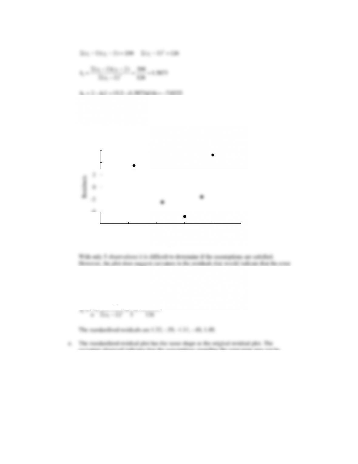
b. The residuals are 3.48, -2.47, -4.83, -1.6, and 5.22
c.
term assumptions are not satisfied. The scatter diagram for these data also indicates that the
underlying relationship between x and y may be curvilinear.
d.
223.78s=
22
2
( ) ( 14)
11
5 126
()
ii
i
x x x
−−
−
The standardized residuals are 1.32, -.59, -1.11, -.40, 1.49.
e. The standardized residual plot has the same shape as the original residual plot. The
curvature observed indicates that the assumptions regarding the error term may not be
satisfied.
46. a.
ˆ2.32 .64yx=+
b.
-6
-4
-2
0
2
4
6
0 5 10 15 20 25
Residuals
x
The assumption that the variance is the same for all values of x is questionable. The variance appears
to increase for larger values of x.
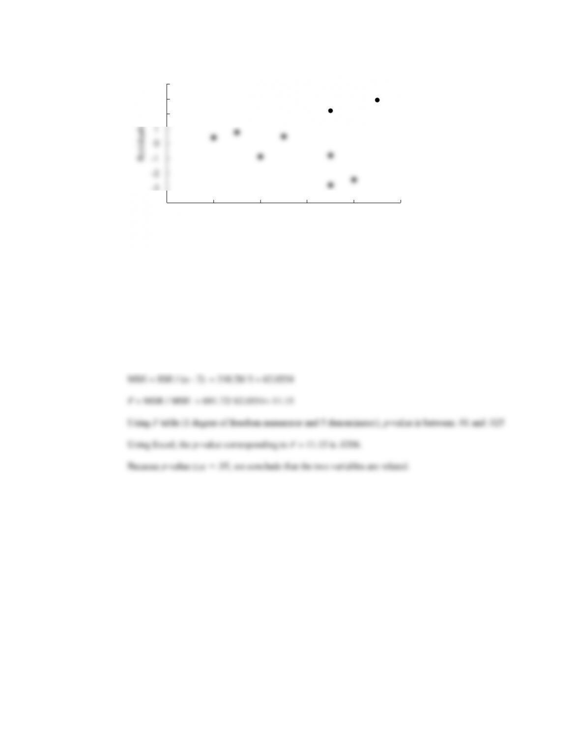
47. a. Let x = advertising expenditures and y = revenue
ˆ29.4 1.55yx=+
b. SST = 1002 SSE = 310.28 SSR = 691.72
MSR = SSR / 1 = 691.72
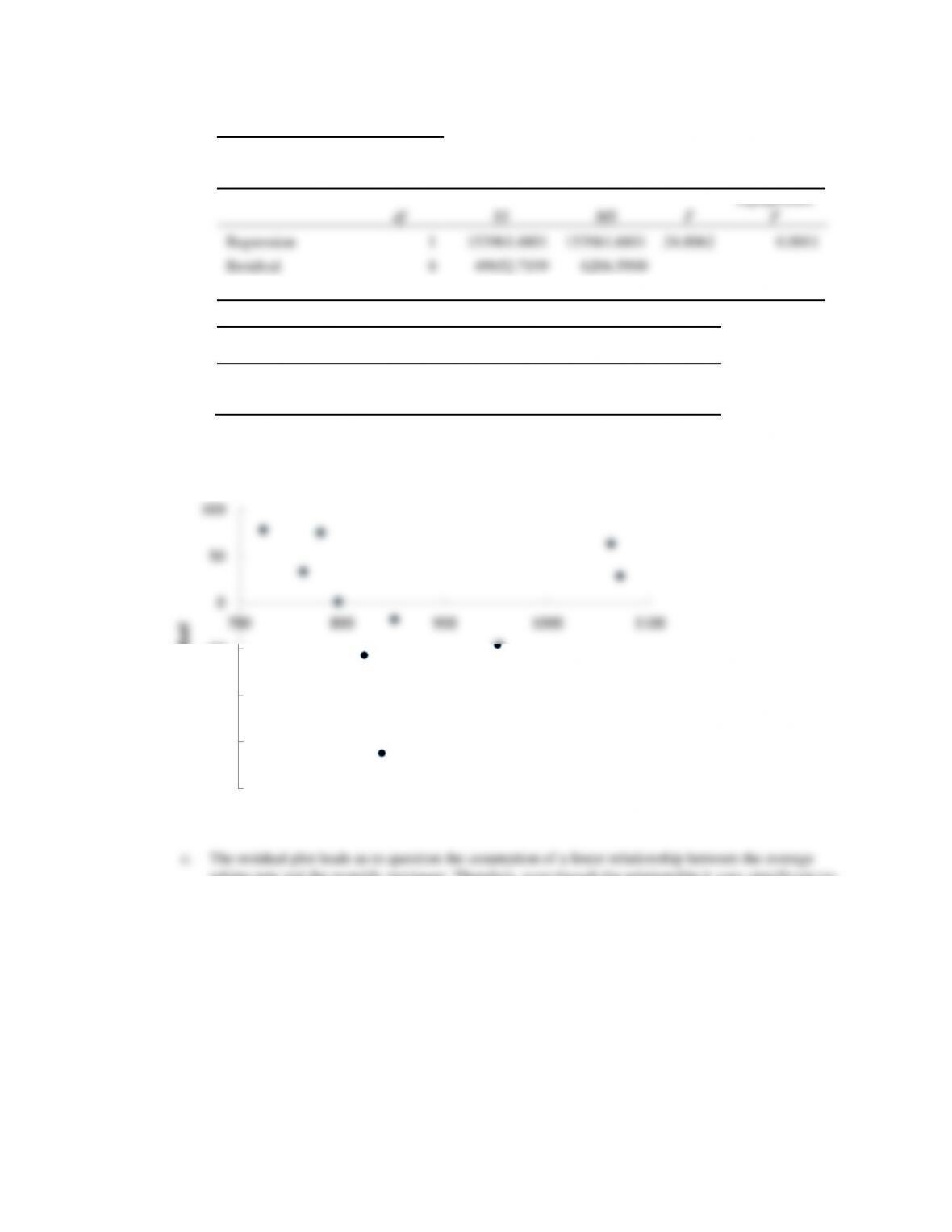
c.
-4
-3
-2
-1
0
1
2
3
4
0 2 4 6 8 10
Residuals
x
d. The residual plot leads us to question the assumption of a linear relationship between x and y. Even
though the relationship is significant at the .05 level of significance, it would be extremely
dangerous to extrapolate beyond the range of the data.
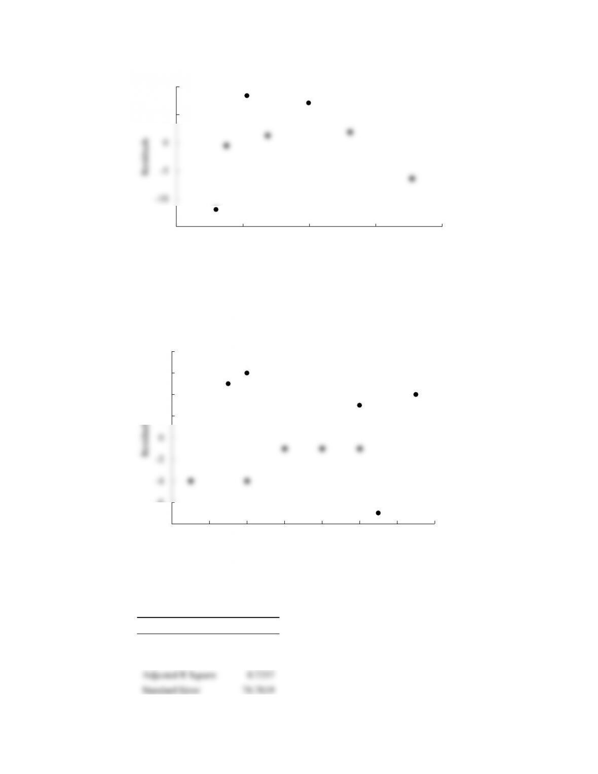
48. a.
ˆ80 4yx=+
b. The assumptions concerning the error term appear reasonable.
49. a. A portion of the Excel output follows:
Regression Statistics
Multiple R
0.8696
R Square
0.7561
Adjusted R Square
0.7257
Standard Error
78.7819
-15
-10
-5
0
5
10
25 35 45 55 65
Residuals
Predicted Values
-8
-6
-4
-2
0
2
4
6
8
0 2 4 6 8 10 12 14
Residuals
x
Observations
10
ANOVA
df
SS
MS
F
Significance
F
Regression
1
153961.6801
153961.6801
24.8062
0.0011
Residual
8
49652.7199
6206.5900
Total
9
203614.4
Coefficients
Standard
Error
t Stat
P-value
Intercept
-197.9583
187.6950
-1.0547
0.3224
Rent ($)
1.0699
0.2148
4.9806
0.0011
ˆ
y
= ˗197.9583 + 1.0699 Rent ($)
b.
asking rent and the monthly mortgage. Therefore, even though the relationship is very significant (p-
value = .0011), using the estimated regression equation to make predictions of the monthly mortgage
beyond the range of the data is not recommended.
50. a. The scatter diagram is shown below:
-200
-150
-100
-50
0
50
100
700 800 900 1000 1100
Residual
Rent ($)
b. Using Excel, the standardized residuals are 2.13, -.90, .14, -.39, -.57, -.04, and -.38. Because the
standard residual for the first observation is greater than 2 it is considered to be an outlier.
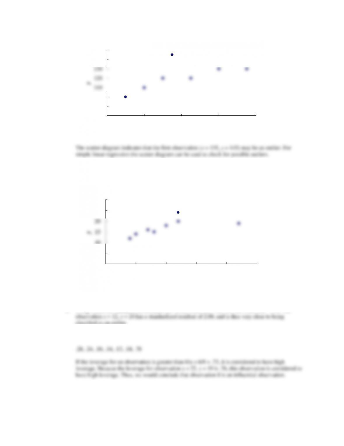
51. a. The scatter diagram is shown below:
The observation x = 22, y = 19 appears to be an influential observation.
b. Using Excel, the standardized residuals are -0.92, -0.38, .01, -.48, .25, .65, 2.00, and –1.14. The
classified as an outlier.
c. Using Excel we obtained the following leverage values:
52. a.
80
90
100
110
120
130
140
150
100 120 140 160 180
y
x
0
5
10
15
20
25
30
0 5 10 15 20 25
y
x
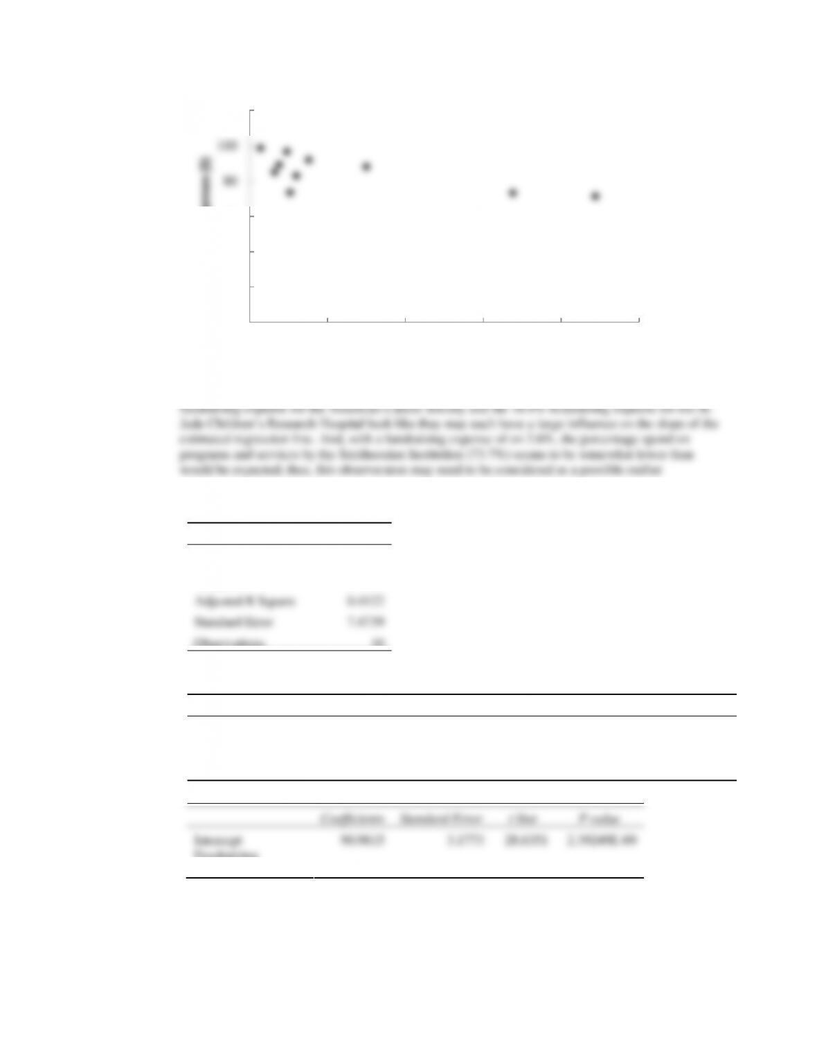
The scatter diagram does indicate potential influential observations. For example, the 22.2%
b. A portion of the Excel output follows:
Regression Statistics
Multiple R
0.6910
R Square
0.4775
Adjusted R Square
0.4122
Standard Error
7.4739
Observations
10
ANOVA
df
SS
MS
F
Significance F
Regression
1
408.3547
408.3547
7.3105
0.0269
Residual
8
446.8693
55.8587
Total
9
855.224
Coefficients
Standard Error
t Stat
P-value
Intercept
90.9815
3.1773
28.6351
2.39249E-09
Fundraising
Expenses (%)
-0.9172
0.3392
-2.7038
0.0269
ˆ
y
= 90.9815 - 0.9172 Fundraising Expenses (%)
0
20
40
60
80
100
120
0 5 10 15 20 25
Program Expenses ($)
Fundraising Expenses (%)
spent on fundraising the percentage spent on program expresses will decrease by .9172%; in other
words, just a little under 1%. The negative slope and value seem to make sense in the context of this
problem situation.
d. The standardized residuals and the values for leverage are shown below.
Charity
Standard Residuals
Leverage
American Red Cross
0.6533
0.1125
World Vision
0.5957
0.1032
Smithsonian Institution
-2.1141
0.1276
Food For The Poor
1.1381
0.1307
American Cancer Society
0.1390
0.6234
Volunteers of America
0.0229
0.1392
Dana-Farber Cancer Institute
-0.6122
0.1447
AmeriCares
1.2007
0.1637
ALSAC - St. Jude Children's Research Hospital
-0.2954
0.3332
City of Hope
-0.7280
0.1219
• Observation 5 (American Cancer Society) is an influential observation becasuse it has high
leverage; leverage = .6234 > 6/10.
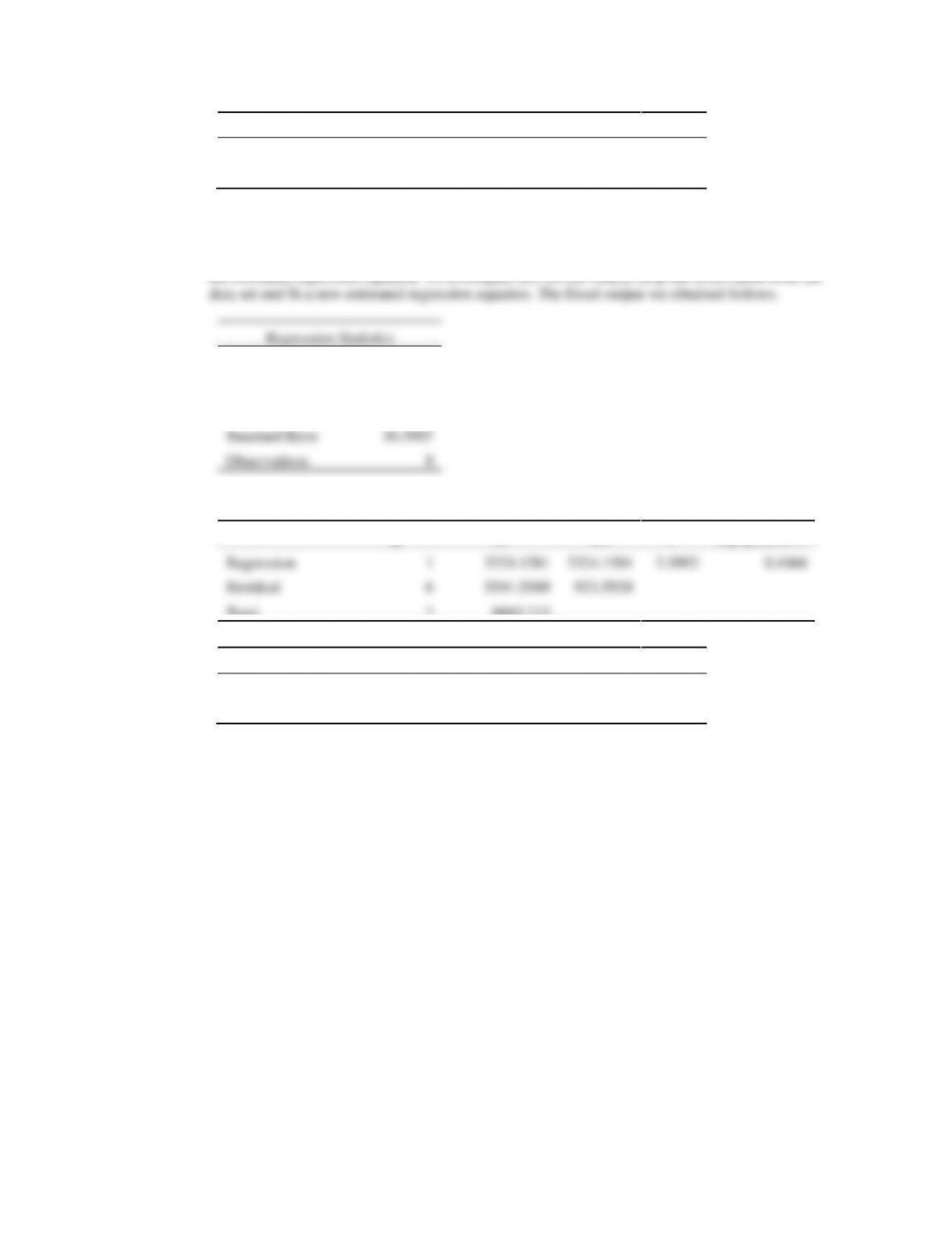
Although fundraising expenses for the Smithsonian Institution are on the low side as compared to
very large value of fundraising expenses for the American Cancer Society suggests that this
obervation has a large influence on the estiamted regresion equation. The following Excel output
shows the results if this observatoin is deleted from the original data.
Regression Statistics
Multiple R
0.5611
R Square
0.3149
Adjusted R Square
0.2170
Standard Error
7.9671
Observations
9
ANOVA
df
SS
MS
F
Significance F
Regression
1
204.1814
204.1814
3.2168
0.1160
Residual
7
444.3209
63.4744
Total
8
648.5022

Coefficients
Standard Error
t Stat
P-value
Intercept
91.2561
3.6537
24.9766
4.207E-08
Fundraising
Expenses (%)
-1.0026
0.5590
-1.7935
0.1160
ˆ
y
= 91.2561 - 1.0026 Fundraising Expenses (%)
The y-intercept has changed slightly, but the slope has changed from -.917 to -1.0026.
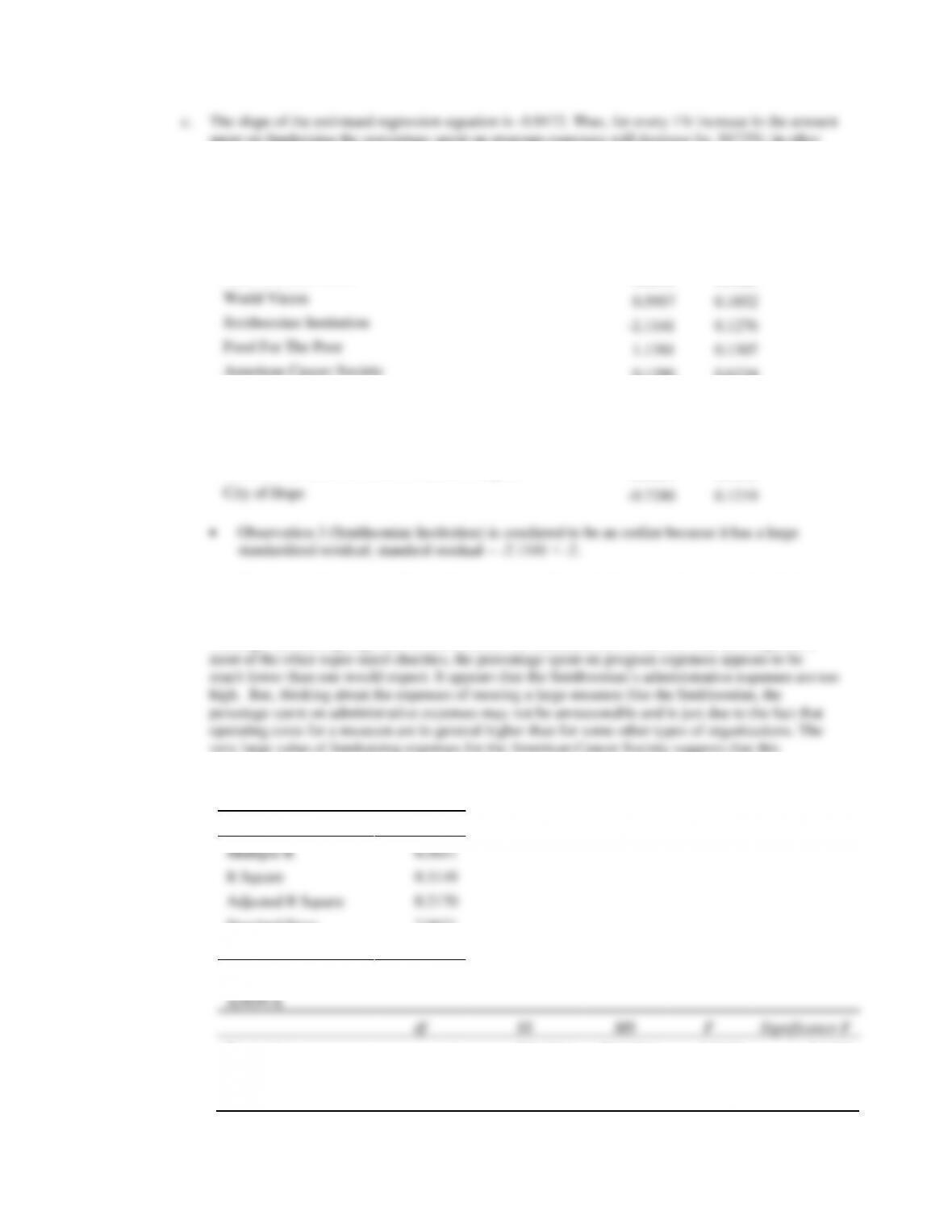
53. a.
b. There appears to be a positive relationship between the two variables. But, observation 9 (U.S.)
appears to be an observation with high leverage and may be very influential in terms of fitting a
linear model to the data.
c. The Excel output follows.
Regression Statistics
Multiple R
0.5097
R Square
0.2598
Adjusted R Square
0.1540
Standard Error
32.0394
Observations
9
ANOVA
df
SS
MS
F
Significance F
Regression
1
2521.9149
2521.9149
2.4568
0.1610
Residual
7
7185.6673
1026.5239
Total
8
9707.5822
0
20
40
60
80
100
120
140
0 100 200 300 400 500 600
Debt/GDP (%)
Gold Value ($B)
Coefficients
Standard Error
t Stat
P-value
Intercept
49.0767
15.1162
3.2466
0.0141
Gold Value
0.1230
0.0785
1.5674
0.1610
ˆ
y
= 49.0767 + 0.1230 Gold Value
d. Looking at the scatter diagram in part (a) it looks like observation 9 will have a lot of influence on


