33.
1.276p=
2.487p=
One week earlier
3.397p=
One month earlier
a. Point estimate:
12
.276 .487 .211pp− = − = −
1 1 2 2
(1 ) (1 ) .276(1 .276) .487(1 .487)
p p p p
−− −−
b. H0: p1 – p3 ≥ 0
Ha: p1 – p3 < 0
c.
1 1 2 3
13
(240)(.276) (240)(.397) .3365
240 240
n p n p
pnn
++
= = =
++
1 1 1 1
34. a.
p1=44/500 =.088
p2=35/300 =.117
p3=36/ 400 =.090
1 2 3 4
Ha: Not all population proportions are equal
Observed Frequencies (fij)
Millionaire
Bridgeport
Los’ Alamos
Naples
Washington
Total
Yes
44
35
36
34
149
No
456
265
364
366
1451
Total
500
300
400
400
1600
Quality
Third
Total
Good
Defective
Total
Quality
Third
Total
Good
Defective
Total
Good
.00
Defective
.01
Millionaire
Bridgeport
Los’ Alamos
Naples
Washington
Total
Yes
46.56
27.94
37.25
37.25
149
No
453.44
272.06
362.75
362.75
1451
Total
500
300
400
400
1600
Chi Square Calculations (fij – eij)2 / eij
Millionaire
Bridgeport
Los’ Alamos
Naples
Washington
Total
Yes
.14
1.79
.04
.28
2.25
No
.01
.18
.00
.03
.23
2=2.48
p2 = population proportion of on-time arrivals for Continental Airlines
p3 = population proportion of on-time arrivals for Delta Air Lines
p4 = population proportion of on-time arrivals for JetBlue Airways
p5 = population proportion of on-time arrivals for Southwest Airlines
p6 = population proportion of on-time arrivals for United Airlines
p7 = population proportion of on-time arrivals for US Airways
a. Point estimates of the population proportion of on-time arrivals for each of these seven airlines are
1
p
= 83/99 = .8384 is the point estimate of the population proportion of on-time arrivals for
American Airlines
2
p
= 54/72 = .75 is the point estimate of the population proportion of on-time arrivals for
Continental Airlines
3
p
= 96/117 = .8205 is the point estimate of the population proportion of on-time arrivals for Delta
Air Lines
p
4
7
p
= 68/80 = .85 is the point estimate of the population proportion of on-time arrivals for US
Airways
b. H0: p1 = p2 = p3 = p4 = p5 = p6 = p7
Ha: Not all population proportions are equal
Observed Frequency (fij)
American
Airlines
Continental
Airlines
Delta Air
Lines
JetBlue
Airways
Southwest
Airlines
United
Airlines
US
Airways
Total
On-Time
Arrivals
83
54
96
60
69
66
68
496
Late Arrivals
16
18
21
22
23
15
12
1277
Totals
99
72
117
82
92
81
80
623
Expected Frequency (eij)
American
Airlines
Continental
Airlines
Delta Air
Lines
JetBlue
Airways
Southwest
Airlines
United
Airlines
US
Airways
Total
On-Time
Arrivals
78.8
57.3
93.1
65.3
73.2
64.5
63.7
496
Late Arrivals
20.2
14.7
23.9
16.7
18.8
16.5
16.3
127
Totals
99
72
117
82
92
81
80
623
Chi Square (fij – eij)2 / eij
American
Airlines
Continental
Airlines
Delta Air
Lines
JetBlue
Airways
Southwest
Airlines
United
Airlines
US
Airways
Total
On-Time
Arrivals
0.22
0.19
0.09
0.43
0.25
0.04
0.29
1.50
Late Arrivals
0.87
0.75
0.34
1.67
0.96
0.14
1.14
5.87
2
= 7.37
Using the
2
table with df = 6,
2
= 7.37 shows the p–value is greater than .10.
Using Excel, the p–value corresponding to
2
= 7.37 is .2880.
p–value > .05, so do not reject H0. We cannot conclude that the population proportion of on-time flights
in 2012 differs for these seven airlines.
p4 = population proportion of visitors who rate the National Gallery as spectacular
p5 = population proportion of visitors who rate the Tate Modern as spectacular
a. Point estimates of the population proportion of visitors who rated each of these museums as
spectacular are
1
p
= 113/150 = .7533 is the point estimate of the population proportion of visitors who rated the
Musée du Louvre as spectacular
2
p
= 94/140 = .6714 is the point estimate of the population proportion of visitors who rated the
Metropolitan Museum of Art as spectacular
3
p
= 96/160 = .60 is the point estimate of the population proportion of visitors who rated the British
p
4
5
p
= 88/110 = .80 is the point estimate of the population proportion of visitors who rated the Tate
Modern as spectacular
b. H0: p1 = p2 = p3 = p4 = p5
Ha: Not all population proportions are equal
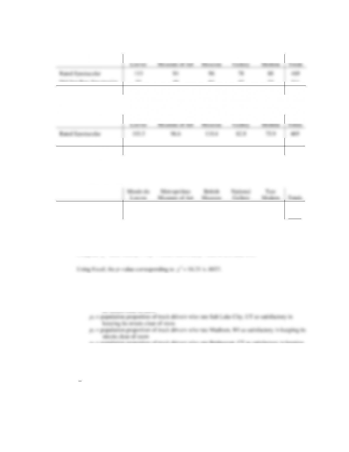
Observed Frequency (fij)
Musée du
Louvre
Metropolitan
Museum of Art
British
Museum
National
Gallery
Tate
Modern
Totals
Rated Spectacular
113
94
96
78
88
469
Did Not Rate Spectacular
37
46
64
42
22
211
Totals
150
140
160
120
110
680
Expected Frequency (eij)
Musée du
Louvre
Metropolitan
Museum of Art
British
Museum
National
Gallery
Tate
Modern
Totals
Rated Spectacular
103.5
96.6
110.4
82.8
75.9
469
Did Not Rate Spectacular
46.5
43.4
49.6
37.2
34.1
211
Totals
150
140
160
120
110
680
Chi Square (fij – eij)2 / eij
Musée du
Louvre
Metropolitan
Museum of Art
British
Museum
National
Gallery
Tate
Modern
Totals
Rated Spectacular
0.88
0.07
1.87
0.27
1.94
5.03
Did Not Rate Spectacular
1.96
0.15
4.15
0.61
4.31
11.18
2
= 16.21
Degrees of freedom = k – 1 = 5 – 1 = 4
Using the
2
table with df = 4,
2
= 16.21 shows the p–value is less than .005.
2
p–value ≤ .05, reject H0. We conclude that the population proportion of visitors who rated the museum
as spectacular differs for these five museums.
38. Let p1 = population proportion of truck drivers who rate Rochester, NY as satisfactory in keeping
p4 = population proportion of truck drivers who rate Bridgeport, CT as satisfactory in keeping
its streets clear of snow
a. Point estimates of the population proportion of truck drivers who rated each of these cities as
satisfactory in keeping its roads clear of snow are
1
p
= 27/48 = .5625 is the point estimate of the population proportion of truck drivers who rated
Rochester, NY as satisfactory in keeping its streets clear of snow
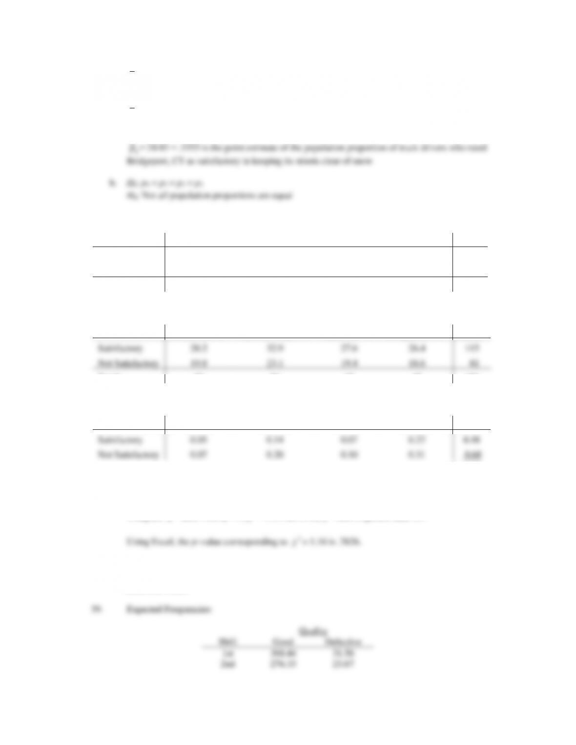
2
p
= 35/56 = .625 is the point estimate of the population proportion of truck drivers who rated Salt
Lake City, UT as satisfactory in keeping its streets clear of snow
3
p
= 29/47 = .617 is the point estimate of the population proportion of truck drivers who rated
Madison, WI as satisfactory in keeping its streets clear of snow
p
4
Observed Frequency (fij)
Rochester, NY
Salt Lake City, UT
Madison, WI
Bridgeport, CT
Totals
Satisfactory
27
35
29
24
115
Not Satisfactory
21
21
18
21
81
Totals
48
56
47
45
196
Expected Frequency (eij)
Rochester, NY
Salt Lake City, UT
Madison, WI
Bridgeport, CT
Totals
Satisfactory
28.2
32.9
27.6
26.4
115
Not Satisfactory
19.8
23.1
19.4
18.6
81
Totals
48
56
47
45
196
Chi Square (fij – eij)2 / eij
Rochester, NY
Salt Lake City, UT
Madison, WI
Bridgeport, CT
Totals
Satisfactory
0.05
0.14
0.07
0.22
0.48
Not Satisfactory
0.07
0.20
0.10
0.31
0.68
2
= 1.16
Degrees of freedom = k – 1 = 4 – 1 = 3
Using the
2
table with df = 3,
2
= 1.16 shows the p–value is greater than .10.
p–value > .05, so do not reject H0. We cannot conclude that the he population proportion of truck
drivers who rate whether the city does a satisfactory job of keeping its streets clear of snow differs for
these four cities.
3rd
184.22
15.78
2
= 8.10
Degrees of freedom = (3 – 1)(2 – 1) = 2
2
2
Using Excel, the p-value corresponding to
2
= 8.10 is .0174.
p–value
.05, reject H0. Conclude that shift and quality are not independent.
Observed
Expected
Frequency
Frequency
Employment
Region
(fi)
(ei)
(fi – ei)2 / ei
Full-Time
Eastern
1105
1046.19
3.31
Full-time
Western
574
632.81
5.46
Part-Time
Eastern
31
28.66
0.19
Part-Time
Western
15
17.34
0.32
Self-Employed
Eastern
229
258.59
3.39
Self-Employed
Western
186
156.41
5.60
Not Employed
Eastern
485
516.55
1.93
Not Employed
Western
344
312.45
3.19
Totals:
2969
23.37
Degrees of freedom = (4 – 1)(2 – 1) = 3
2
2
Using Excel, the p-value corresponding to
2
= 23.37 is .0000.
p-value
.05, reject H0. Conclude that employment status is not independent of region.
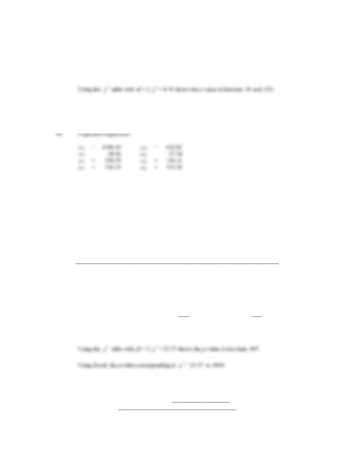
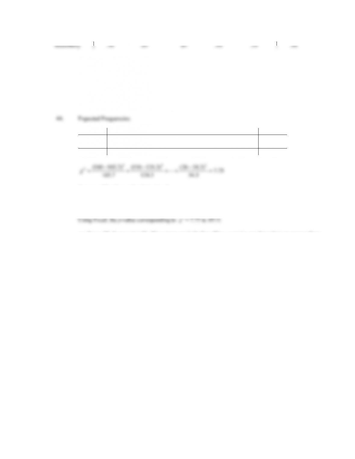
41. Expected frequencies:
Loan Approval Decision
Loan Offices
Approved
Rejected
Miller
24.86
15.14
McMahon
18.64
11.36
Games
31.07
18.93
Runk
12.43
7.57
2
= 2.21
Degrees of freedom = (4 – 1)(2 – 1) = 3
Using the
2
table with df = 3,
2
= 1.21 shows the p-value is greater than .10.
p–value > .05, do not reject H0. The loan decision does not appear to be dependent on the
officer.
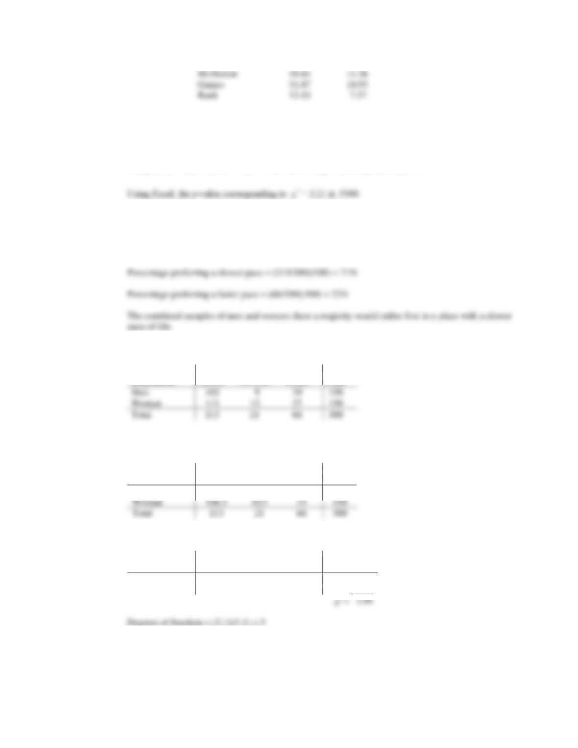
42. a. Column totals: Slower 213, No Preference 21, and Faster 66.
b. Observed Frequency (fij)
Preferred Pace of Life
Respondent
Slower
No Pref
Faster
Total
Men
102
9
39
150
Woman
111
12
27
150
Total
213
21
66
300
Expected Frequency (eij)
Preferred Pace of Life
Respondent
Slower
No Pref
Faster
Total
Men
106.5
10.5
33
150
Woman
106.5
10.5
33
150
Total
213
21
66
300
Chi Square (fij – eij)2/ eij
Preferred Pace of Life
Respondent
Slower
No Pref
Faster
Total
Men
.19
.21
1.09
1.495
Woman
.19
..21
1.09
1.495
χ2 = 2.99
Degrees of freedom = (2-1)(3-1) = 2
Using the
2
table with df = 2,
2
= 2.99 shows the p-value is greater than .10.
Using Excel, the p-value corresponding to
2
= 2.99 is .2242.
p-value > .05, do not reject H0. We cannot reject the assumption that the preferred pace of life is
conclude men and women differ with respected to the preferred pace of life.
This is a good example of where it would be desirable to study this further before drawing a conclusion.
Including a larger number of men and women in the sample and repeating the analysis should be
considered.
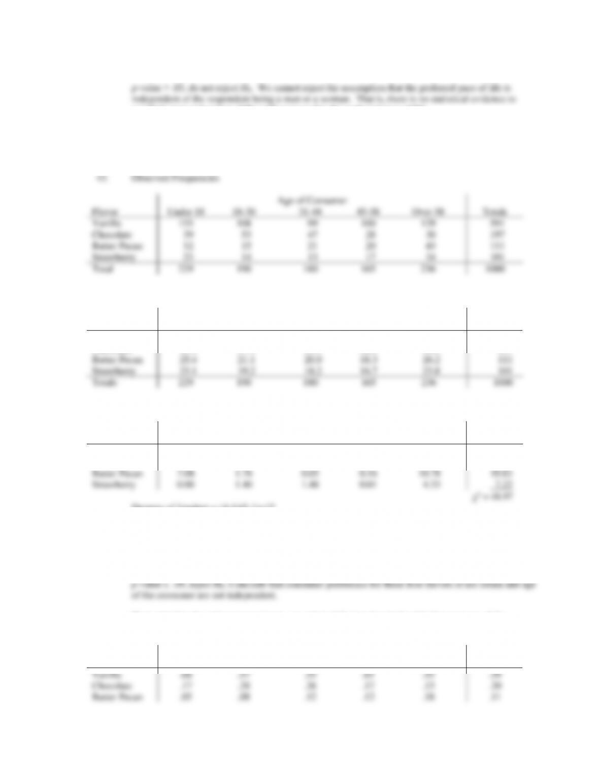
Age of Consumer
Flavor
Under 18
18–30
31–44
45–58
Over 58
Totals
Vanilla
155
108
99
100
129
591
Chocolate
39
53
47
28
30
197
Butter Pecan
12
15
21
20
43
111
Strawberry
23
14
13
17
34
101
Total
229
190
180
165
236
1000
Expected Frequencies
Age of Consumer
Flavor
Under 18
18–30
31–44
45–58
Over 58
Totals
Vanilla
135.3
112.3
106.4
97.5
139.5
591
Chocolate
45.1
37.4
35.5
32.5
46.5
197
Butter Pecan
25.4
21.1
20.0
18.3
26.2
111
Strawberry
23.1
19.2
18.2
16.7
23.8
101
Totals
229
190
180
165
236
1000
Chi Square
Age of Consumer
Flavor
Under 18
18–30
31–44
45–58
Over 58
Totals
Vanilla
2.86
0.16
0.51
0.06
0.79
4.38
Chocolate
0.83
6.48
3.76
0.62
5.85
17.54
Butter Pecan
7.08
1.76
0.05
0.16
10.78
19.83
Strawberry
0.00
1.40
1.48
0.01
4.33
7.22
2 = 48.97
Degrees of freedom = (4-1)(5-1)=12
Using the
2
table with df = 12,
2
= 48.97 shows the p-value is less than .005.
Using Excel, the p-value corresponding to
2
= 48.97 is approximately 0.
If we calculate the column percentages, we gain insight into the relationship between age of the
consumer and the preferred ice cream flavor.
Age of Consumer
Flavor
Under 18
18–30
31–44
45–58
Over 58
Totals
Vanilla
.68
.57
.55
.61
.55
.59
Chocolate
.17
.28
.26
.17
.13
.20
Butter Pecan
.05
.08
.12
.12
.18
.11
Strawberry
.10
.07
.07
.10
.14
.10
The proportion of consumers who prefer butter pecan is much higher in the Over 58 group that (.18)
than in the entire sample (.11), and the proportion of consumers who prefer butter pecan is much lower
in the Under 18 group (.05). There is also a great deal of difference in reference for chocolate between
some of these groups; the proportion of consumers who chocolate is much lower in the Over 58 group
that (.13) than in the entire sample (.20), and the proportion of consumers who prefer chocolate is much
higher in the 18 -30 group (.28) and the 31-44 group (.26). Butter pecan ice cream is favored by older
consumers, while chocolate is favored by consumers who are between 18 and 44 years old.
Los Angeles
San Diego
San Francisco
San Jose
Totals
Occupied
165.7
124.3
186.4
165.7
642
Vacant
34.3
25.7
38.6
34.3
133
Totals
200.0
150.0
225.0
200.0
775
Degrees of freedom = (2 – 1)(4 – 1) = 3
Using the
2
table with df = 3,
2
= 7.75 shows the p-value between .05 and .10.
2
p-value > .05, do not reject H0. We cannot conclude that office vacancies are dependent on metropolitan
area, but it is close: the p-value is slightly larger than .05.