
Chapter 11
Comparisons Involving Proportions and a
Test of Independence
Learning Objectives
1. Be able to develop interval estimates and conduct hypothesis tests about the difference between the
proportions of two populations.
2. Know the properties of the sampling distribution of the difference between two proportions
( )p p
1 2
−
.
3. Be able to conduct hypothesis tests about the difference between the proportions of three or more
populations.
4. For a test of independence, be able to set up a contingency table, determine the observed and
expected frequencies, and determine if the two variables are independent.
5. Understand the role of the chi-square distribution in conducting the tests in this chapter and be able
to compute the chi-square test statistic for each application.
Solutions:
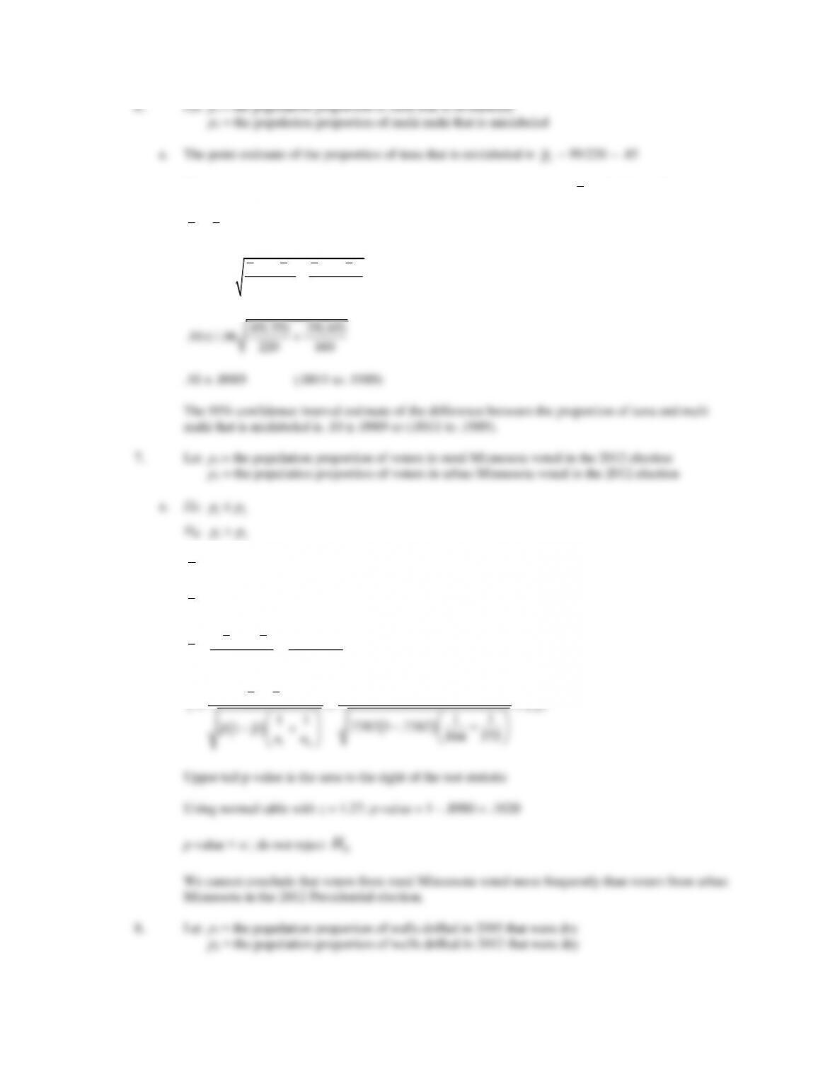
1. a.
12
pp−
= .48 – .36 = .12
b.
1 1 2 2
1 2 .05
12
(1 ) (1 )p p p p
p p z nn
−−
− +
.48(1 .48) .36(1 .36)
−−
2. a.
1 1 2 2
12
100(.28) 140(.20) .2333
100 140
n p n p
pnn
++
= = =
++
b.
( ) ( )
12
12
.28 .20 1.44
11
11 .2333 1 .2333
1100 140
pp
z
pp
nn
−−
= = =
−+
−+

p – value = 2(1 – .9251) = .1498
c. p-value > .05; do not reject H0. We cannot conclude that the two population proportions
differ.
3. a.
1 1 2 2
12
200(.22) 300(.16) .1840
200 300
n p n p
pnn
++
= = =
++
( ) ( )
12
12
.22 .16 1.70
11
11 .1840 1 .1840
1200 300
pp
z
pp
nn
−−
= = =
−+
−+
1 1 2 2
1 2 .025
12
(1 ) (1 )p p p p
p p z nn
−−
− +
.55(1 .55) .48(1 .48)
.55 .48 1.96 400 400
−−
− +
.07 .0691 (.0009 to .1391)
b. The point estimate of the proportion of men who trust recommendations made on Pinterest is
2
p
=
102/170 = .60
c.
12
pp−
= .78 – .60 = .18
1 1 2 2
.025
12
(1 ) (1 )
.18 p p p p
znn
−−
+

12
12
b.
1
p
= 24/119 = .2017
c.
2
p
= 21/162 = .1111
d.
1 1 2 2
12
24 18 .1495
119 162
n p n p
pnn
++
= = =
++
( ) ( )
12
12
.2017 .1111 2.10
11
11 .1495 1 .1495
1119 162
pp
z
pp
nn
−−
= = =
−+
−+
b.
p1
= 104/200 = .52 (52%)
2
p
= 74/200 = .37 (37%)
c.
p=n1p1+n2p2
n1+n2
=104 +74
200 +200 =.445
z=p1–p2
p1–p
( )
1
n1
+1
n2
æ
è
çö
ø
÷
=.52–.37
.445 1–.445
( )
1
200 +1
200
æ
è
çö
ø
÷
=3.02
12
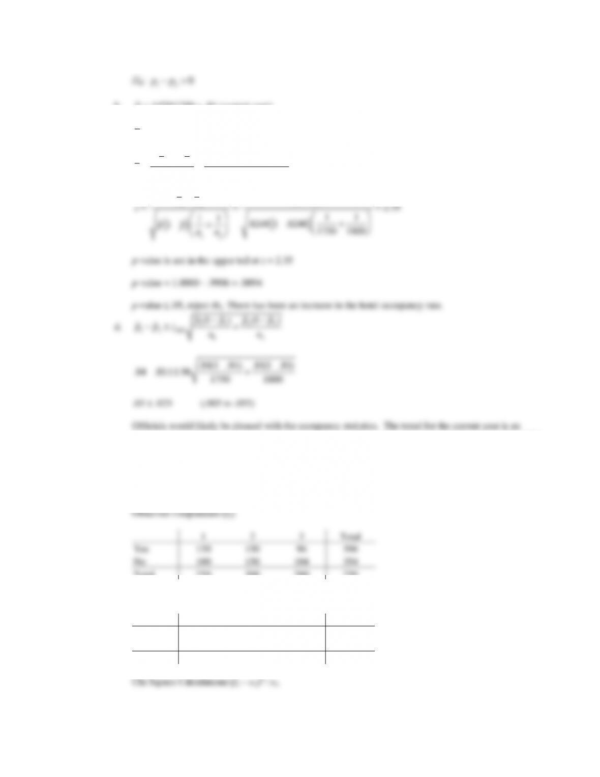
b.
1
p
= 1470/1750 = .84 (current year)
2
p
= 1458/1800 = .81 (previous year)
c.
p=n1p1+n2p2
n1+n2
=1750(.84)+1800(.81)
1750 +1800 =.8248
increase in hotel occupancy rates compared to last year. The point estimate is a 3% increase with a 95%
confidence interval from .5% to 5.5%.
11. H0:
1 2 3
p p p==
Ha: Not all population proportions are equal
1
2
3
Total
Yes
150
150
96
396
No
100
150
104
354
Total
250
300
200
750
Expected Frequencies (eij)
1
2
3
Total
Yes
132.0
158.4
105.6
396
No
118.0
141.6
94.4
354
Total
250
300
200
750

1
2
3
Total
Yes
2.45
.45
.87
3.77
No
2.75
.50
.98
4.22
2
= 7.99
Using the
2
table with df = 2,
2
= 7.99 shows the p–value is between .025 and .01
Using Excel, the p–value corresponding to
2
= 7.99 is .0184
12. a.
p1=150 /250 =.60
p2=150 /300 =.50
2
2
2
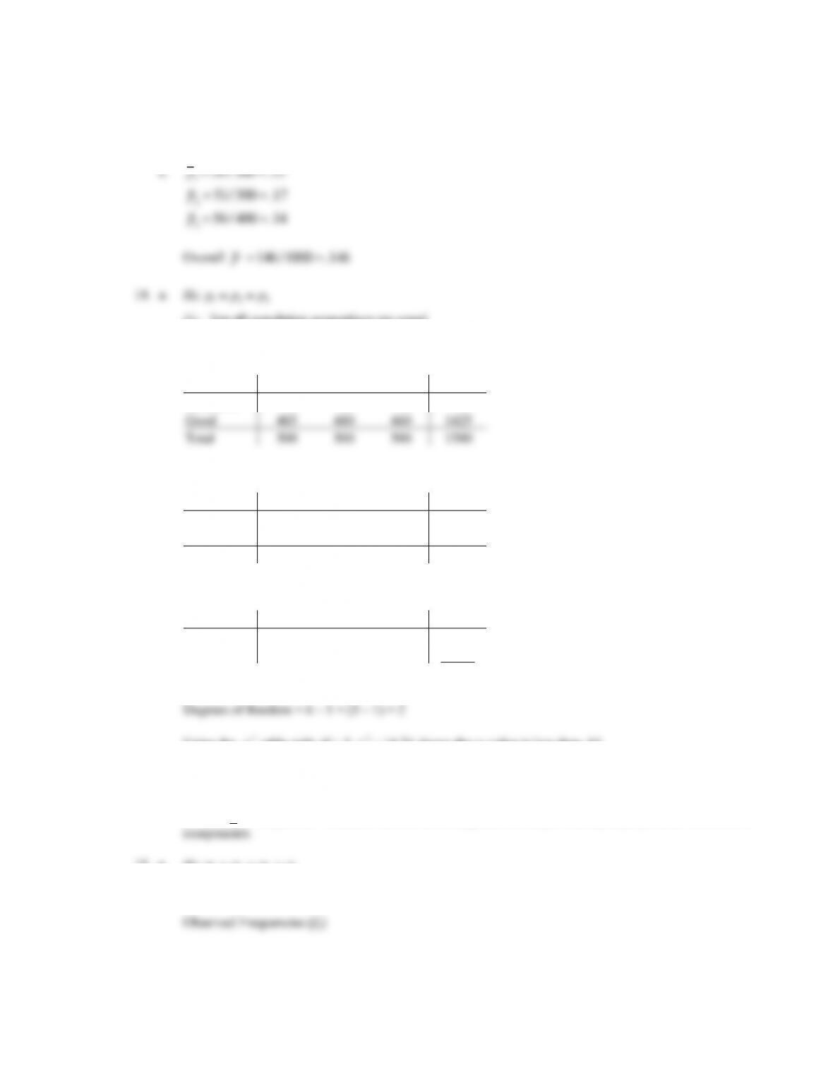
p–value > .05, do not reject H0. We are unable to reject the null hypothesis that the population
proportions are the same.
1 2 3
Ha: Not all population proportions are equal
b. Observed Frequencies (fij)
Component
A
B
C
Total
Defective
15
20
40
75
Good
485
480
460
1425
Total
500
500
500
1500
Expected Frequencies (eij)
Component
A
B
C
Total
Defective
25
25
25
75
Good
475
475
475
1425
Total
500
500
500
1500
Chi Square Calculations (fij – eij)2 / eij
Component
A
B
C
Total
Defective
4.00
1.00
9.00
14.00
Good
.21
.05
.47
0.74
2
= 14.74
Using the
2
table with df = 2,
2
= 14.74 shows the p–value is less than .01
Using Excel, the p–value corresponding to
2
= 14.74 is .0006
p–value < .05, reject H0. Conclude that the three suppliers do not provide equal proportions of defective
15. a. H0:
1 2 3 4
p p p p= = =
Ha: Not all population proportions are equal
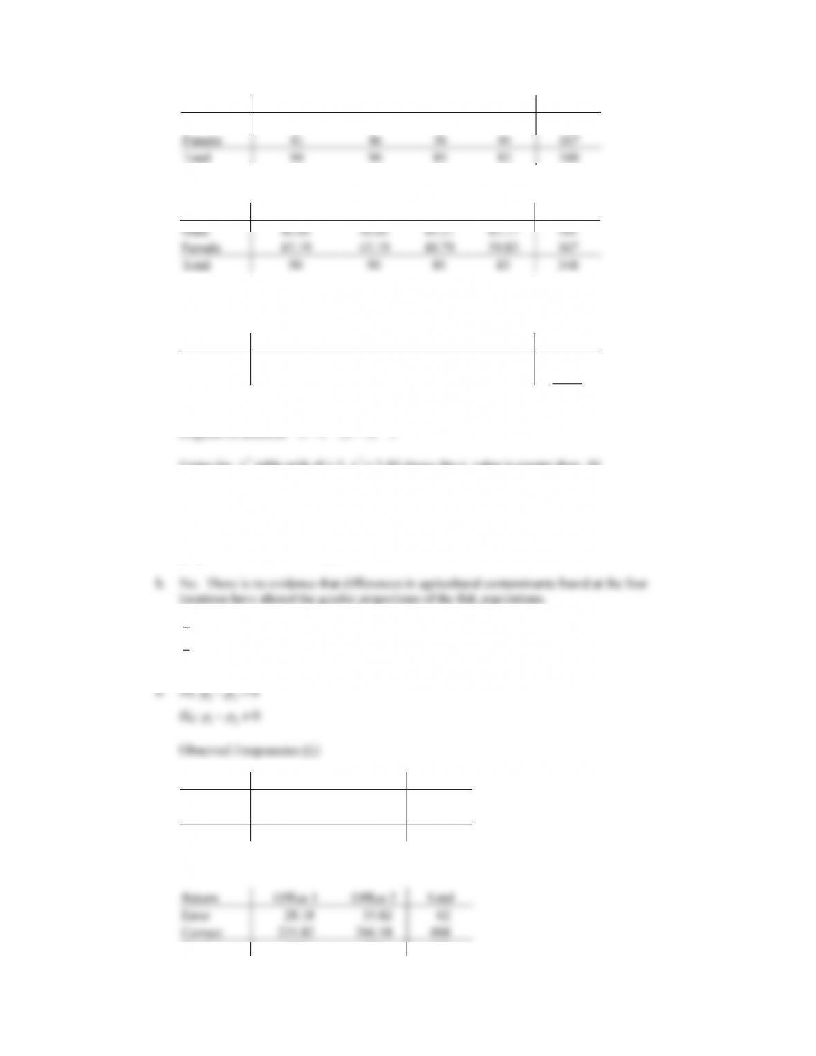
Expected Frequencies (eij)
Female
41
46
36
44
167
Gender
A
B
C
D
Total
Male
46.81
46.81
44.21
43.17
181
Female
43.19
43.19
40.79
39.83
167
Total
90
90
85
83
348
Chi Square Calculations (fij – eij)2 / eij
Gender
A
B
C
D
Total
Male
.10
.17
.52
.40
1.19
Female
.11
.18
.56
.44
1.29
c
2=2.49
Degrees of freedom = k – 1 = (4 – 1) = 3
Using the
2
table with df = 3,
2
= 2.49 shows the p–value is greater than .10
Using Excel, the p–value corresponding to
2
= 2.49 is .4771
p–value > .05, do not reject H0. Conclude that we are unable to reject the hypothesis that the population
proportion of male fish is equal in all four locations.
16. a.
p1=35/250 =.14
14% error rate
p2=27 / 300 =.09
9% error rate
Return
Office 1
Office 2
Total
Error
35
27
62
Correct
215
273
488
Total
250
300
550
Expected Frequencies (eij)
Return
Office 1
Office 2
Total
Error
28.18
33.82
62
Correct
221.82
266.18
488
Total
250
300
550
Gender
A
B
C
D
Total
Male
49
44
49
39
181
Total
90
90
85
83
348

Chi Square Calculations (fij – eij)2 / eij
Return
Office 1
Office 2
Total
Error
1.65
1.37
3.02
Correct
.21
.17
.38
2
= 3.41
df = k – 1 = (2 – 1) = 1
Using the
2
table with df = 1,
2
= 3.41 shows the p–value is between .10 and .05
2
p–value < .10, reject H0. Conclude that the two offices do not have the same population proportion
error rates.
c. With two populations, a chi–square test for equal population proportions has 1 degree of freedom. In
this case the test statistic
c
2
is always equal to z2. This relationship between the two test statistics
hypothesis tests about the equality of the two population proportions.
17. a. H0:
1 2 3 4
p p p p= = =
Ha: Not all population proportions are equal
Social Net
Great Britain
Israel
Russia
USA
Total
Yes
344
265
301
500
1410
No
456
235
399
500
1590
Total
800
500
700
1000
3000
Social Net
Great Britain
Israel
Russia
USA
Total
Yes
376
235
329
470
1410
No
424
265
371
530
1590
Total
800
500
700
1000
3000
Chi Square Calculations (fij – eij)2 / eij
Social Net
Great Britain
Israel
Russia
USA
Total
Yes
2.72
3.83
2.38
1.91
10.85
No
2.42
3.40
2.11
1.70
9.62
c
2=20.47
Degrees of freedom = df = k – 1 = (4 – 1) = 3
Using the
2
table with df = 3,
2
= 20.47 shows the p–value is less than .01
2
p–value
.05, reject H0. Conclude the population proportions are not all equal.
b. Great Britain 344/800 = .43
Israel 265/500 = .53 (Largest with 53% of adults)
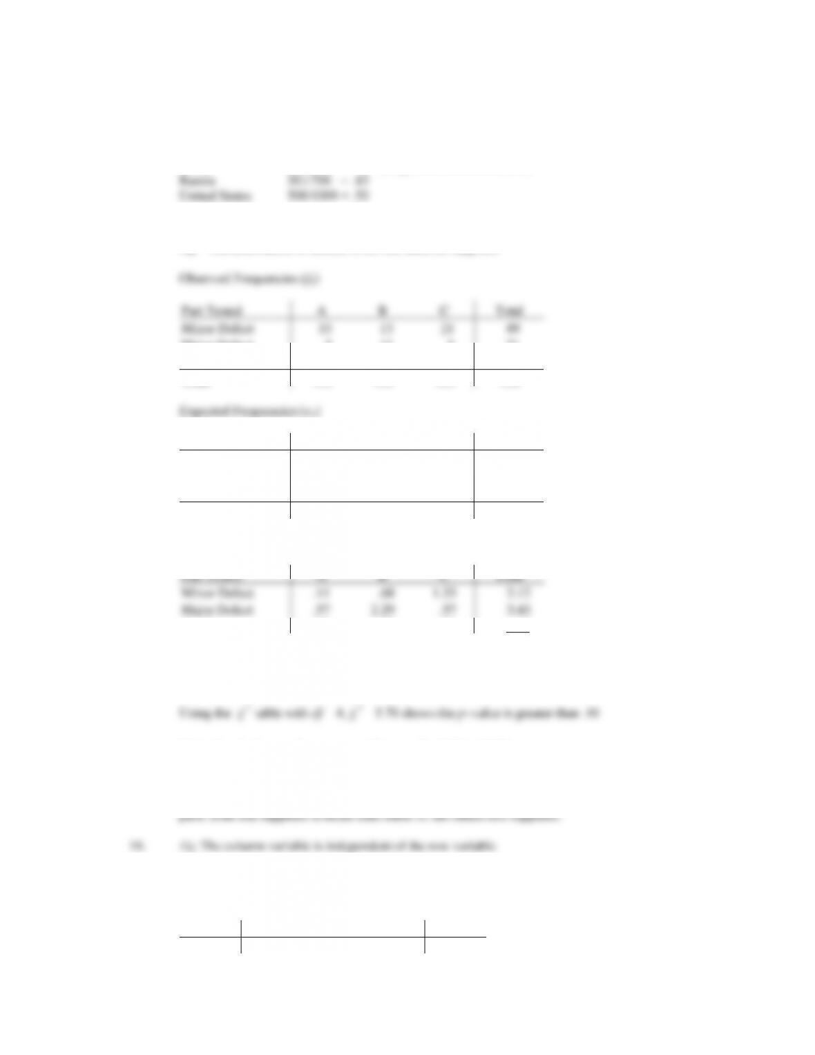
18. H0: The distribution of defects is the same for all suppliers
Ha: The distribution of defects is not the same all suppliers
Part Tested
A
B
C
Total
Minor Defect
15
13
21
49
Major Defect
5
11
5
21
Good
130
126
124
380
Total
150
150
150
450
Part Tested
A
B
C
Total
Minor Defect
16.33
16.33
16.33
49
Major Defect
7.00
7.00
7.00
21
Good
126.67
126.67
126.67
380
Total
150
150
150
450
Chi Square Calculations (fij – eij)2 / eij
Part Tested
A
B
C
Total
Minor Defect
.11
.68
1.33
2.12
Major Defect
.57
2.29
.57
3.43
Good
.09
.00
.06
.15
2
= 5.70
Degrees of freedom = (r – 1)(k – 1) = (3 – 1)(3 – 1) = 4
2
2
Using Excel, the p–value corresponding to
2
= 5.70 is .2227
p–value > .05, do not reject H0. Conclude that we are unable to reject the hypothesis that the
population distribution of defects is the same for all three suppliers. There is no evidence that quality of
Ha: The column variable is not independent of the row variable
Observed Frequencies (fij)
A
B
C
Total
P
20
44
50
114
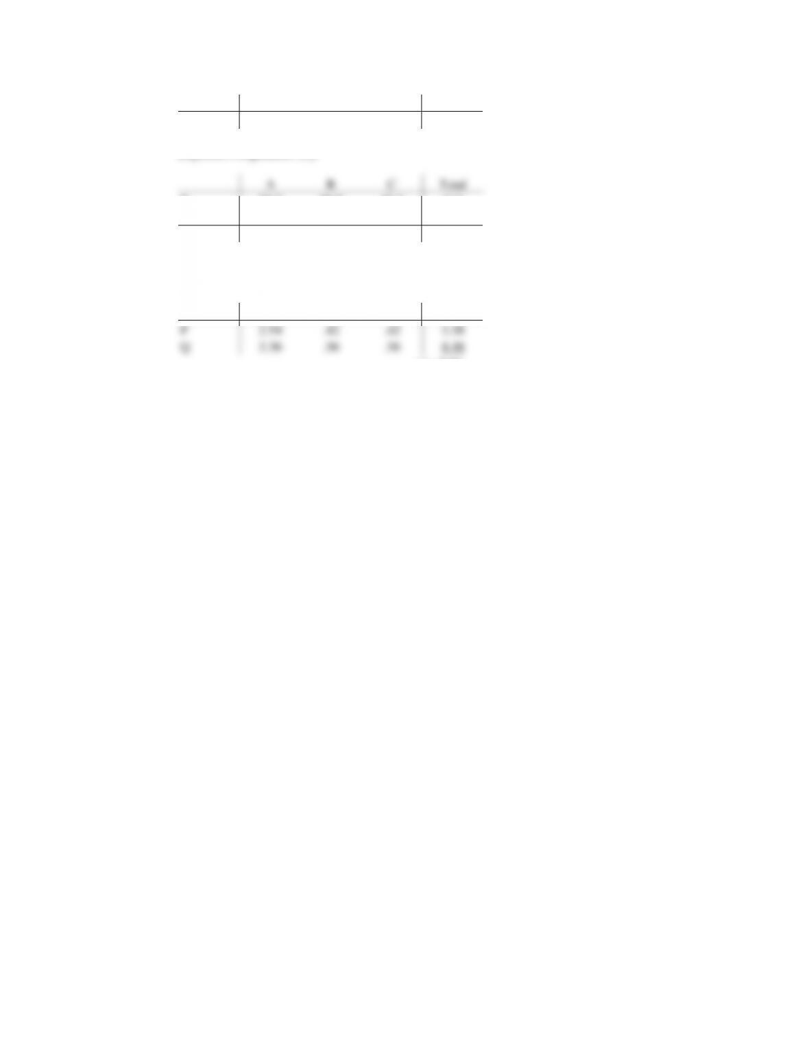
Q
30
26
30
86
Total
50
70
80
200
Expected Frequencies (eij)
P
114
Q
Total
50
70
80
200
P
Q