Answers to Back-of-the-Chapter Problems
1. Survey methods are relatively inexpensive but are subject to potential
problems: sample bias, response bias, and response accuracy. Test
marketing avoids these problems by providing data on actual consumer
2. a. Coca Cola’s management is likely to conclude that consumers will
b. Yes, these rankings are consistent with the information in part (a).
Consumers prefer Pepsi to Coke Classic by 58 to 42 (types A and C)
c. It would be a big mistake to replace Classic by New Coke. The obvious
strategy is to retain Classic but also offer and promote New Coke. New
Coke will attract type C consumers away from Pepsi. As the text
3. a. Northwest does have a better overall on-time record than Delta. Its
b. Delta’s management will tout city-by-city on-time comparisons. In New
York, its frequency of late flights is: 484/1,987 = .24 or 24 percent,
John Wiley & Sons
4-1
c. The disaggregate comparisons provide the more accurate measure of
on-time performance. Here, Delta wins hands down. The overall record
is misleading. Delta’s overall on-time percentage looks worse because it
4. a. False. A high R2 indicates that the equation closely tracks the past data,
but this is only one part of performance. A complete evaluation would
b. Partly True. More data is better as long as the time-series relationship
is stable. However, such behavior often changes over time. If two time
c. False. Throwing in everything but the kitchen sink is bad on theoretical
grounds and empirical grounds. Including irrelevant or insignificant
d. Partly True. But there are exceptions. i) Even forecasts that accurately
track the past can produce implausible long-term predictions. ii) No
b. This coefficient measures the price elasticity of demand, EP = -.29. A 20
John Wiley & Sons
4-2
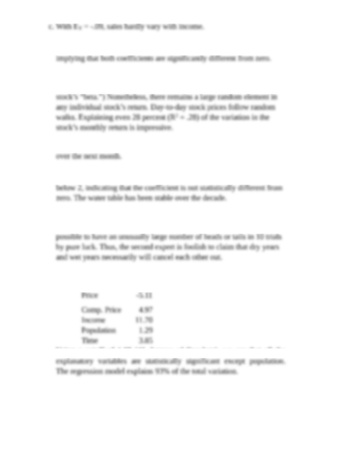
6. a. Both t-values (based on 60 months of data) are much greater than 2,
b. The equation says that the expected return on Pepsi’s stock roughly
follows the expected return on the S&P 500. (The coefficient .92 is the
c. Setting RS&P = -1 implies RPEP = .06 – .92 = -.86 percent expected return
7. a. Although the time coefficient is negative (b = -.4), its t-value is well
b. Think of yearly rainfall as one thinks of tosses of a coin. Even though
each coin toss is random and independent of the other tosses, it is still
8. a. The t-statistics for each of the explanatory variables are:
Using a cutoff of 1.68 (41 degrees of Freedom), we see that all the
b. Price elasticity is (dQ/dP)(P/Q) = (-3,590.6)(7.50/20,000) = -1.35.
John Wiley & Sons
4-3
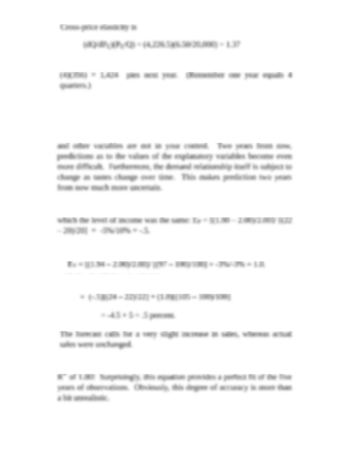
c. According to the regression, pie sales should increase by approximately
d. You might be fairly confident in predicting sales for the next quarter
given that 93% of the variation is explained by the regression but only
if accurate information about the explanatory variables can be obtained.
Of course, you control your own price. However, competitors’ prices
9. a. To estimate price elasticity, we compare 2011 and 2014, two years in
b. Comparing 2011 and 2013 when prices were constant, we find:
c. dQ/Q = EP(dP/P) + EY(dY/Y)
d. The OLS regression produces the equation: Q = 1 – .05P + .02Y with an
John Wiley & Sons
4-4
b. The second manager is correct in principle. Using the average change
b. Although the equation’s R2 is .69, the t-value on the time trend is only
c. Suppose you take the estimated coefficient at face value (even though it
lacks statistical significance.) Then, the forecast for year 5 is 95 + (5.5)
12. a. As the economy improves, we would expect firms to stop laying off
b. Yacht sales probably will not rebound until well after the upswing is
13. a. Yes, the equation makes economic sense. Growth in tire sales is fueled
b. The equation performs well in explaining the past data (R2 = .83).
John Wiley & Sons
4-5
(1.12 – 1)/.41 = .29. The first coefficient is significantly different than
d. The forecast is: .45 + (1.41)(-2) + (1.12)(-13) = -16.93. An actual drop
Discussion Question
One way of comparing the qualitative and quantitative approaches is to put
them to a side-by-side forecasting test. Ask each approach to make forecasts
Another powerful test is to combine the approaches in estimating movie
demand. While human decision makers might be skilled at identifying
important qualitative factors, they are less competent in estimating the
magnitude of these factors’ impacts on demand. This is where statistical
Spreadsheet Problems
S1. a. The OLS estimated equation is: W = 18.25 – .41t, where the t-statistic
associated with the “year” coefficient is -1.616. This t-value fails
John Wiley & Sons
4-6
b. Average rainfall in the last 5 years was 46 inches compared to 38.4
inches in the first 5 years. Thus, accounting for variation in rainfall is
c. The multiple regression equation is:
W = 9.69 – .51t + .216R.
This equation (with an R2 of .82) provides a much better fit to the data
S2. a. The estimated OLS equation is: Q = 332.5 – 506.6P. The equation is
c. The Log-Log equation is:
This provides a better fit of the data (R2 = .992) than the linear
equation. The Log-Log equation implies the demand equation:
S3 a. The OLS regression equation is: Q = 95.0 + 4.68t. The coefficient for
b. The constant-growth equation is estimated in the logarithmic form:
John Wiley & Sons
4-7
The coefficient of Log(t) is highly significant. The growth equation
provides a slightly better fit (R2 = .996) than the linear equation and
c. The linear equation’s predictions are: 179.2, 183.9, 188.6, and 193.3.
S4 a. For the years 1975-2006, neither a linear time trend nor an exponential
time trend provides a particularly good fit. This should be evident from
b. Dividing the sample at 1996 makes sense. The linear regression for the
years up to 1996 shows no statistically significant trend upward or
downward – that is, the coefficient for the yearly effect is no different
than zero. The best fitted equation is simply: P = 112.0. Between 1996
Two Extra Spreadsheet Problems
E1. There is considerable debate within your firm concerning the effect of
advertising on sales. The marketing department believes advertising has
a large positive effect; others are not so sure. For instance, the
John Wiley & Sons
4-8
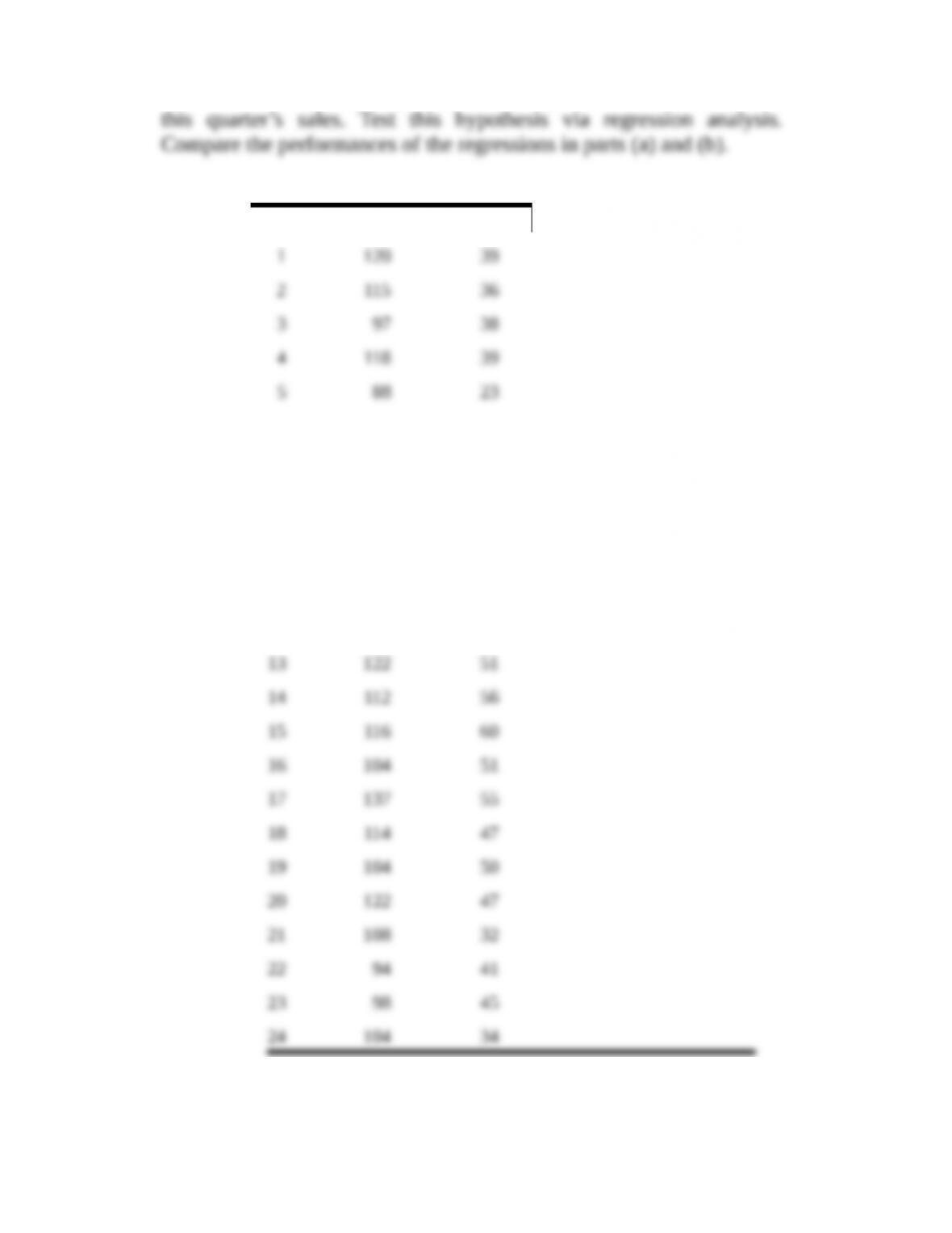
b. Others in the company argue that the last quarter’s sales best predict
Quarter Unit Sales Advertising
6 63 22
7 82 40
8 80 42
9 95 36
10 106 49
11 105 66
12 136 65
John Wiley & Sons
4-9
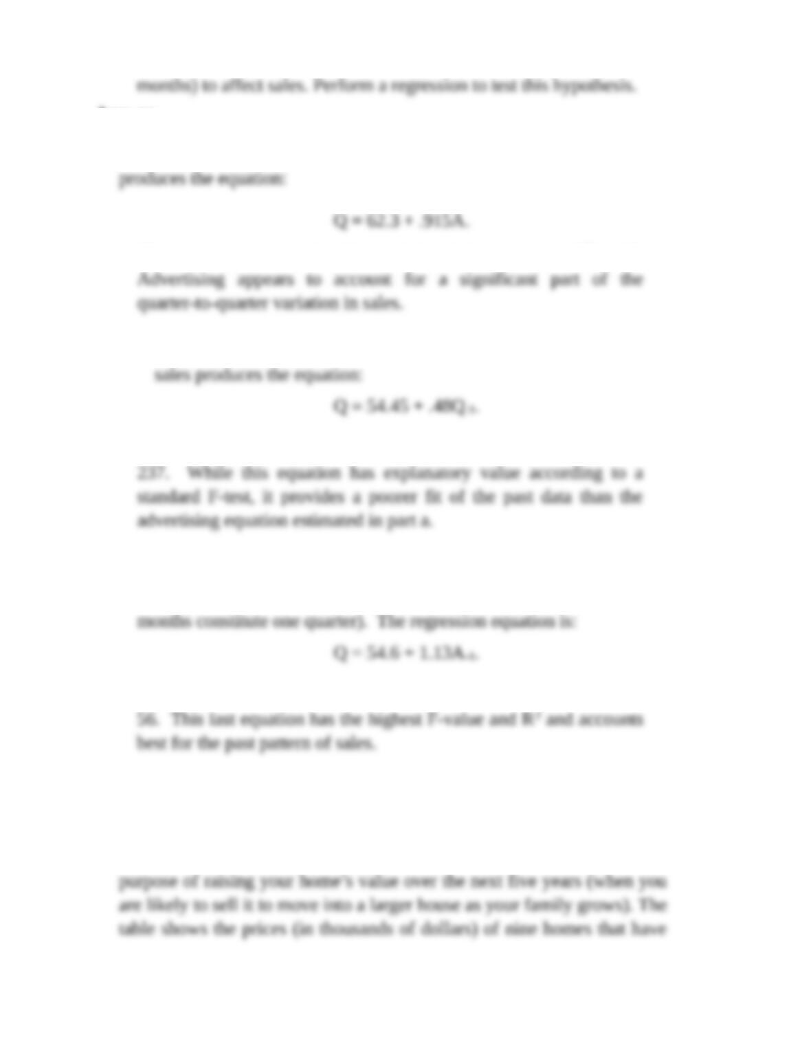
c. Some believe the impact of advertising takes time (as long as three
Answer
a. A regression of unit sales against the current level of advertising
The t-statistic associated with A is 3.6 and the equation’s R2 is .37.
b. A regression of this quarter’s unit sales against the last quarter’s
The t-statistic associated with Q-1 is 2.55 and the equation’s R2 is .
c. To test the lagged effect, we regress Q against A-1 (since three
The t-statistic associated with A-1 is 5.20, and the equation’s R2 is .
E2. You live in a neighborhood development of very similar homes (roughly
the same floor plans and lot sizes). You are considering possible home
improvements, not only for their immediate value to you but also for the
John Wiley & Sons
4-10

a. Compute a multiple-regression equation estimating a typical home’s
sales price based on the various improvements. (Hint: Begin by
Selling
Price
New
Bathroom
New
Kitchen
Landscaping
and Patio Pool
Central Air
Conditioning
b. Which improvements make a significant positive difference in the
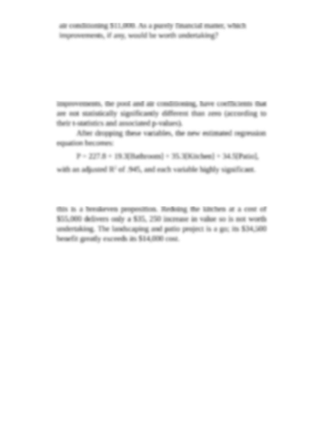
c. In exploring the costs of making the various improvements, you have
1 This problem was inspired by J. Toczek, “Home Improvement,” ORMS Today (October 2010): p. 12.
John Wiley & Sons
4-11
Answer
a. and b. A regression of house values (column D) against the dummy
variables for all five improvements (columns E through I) generates
a high F-value and a high adjusted R2 of .96. However, the last two
c. Redoing the bathroom raises the home’s value by $19,300 and by
coincidence costs almost exactly the same amount ($19,000). So
John Wiley & Sons
4-12