11.27 Between 1980 and 2000, the average CO emission factor of the vehicle fleet in
Hillsborough County, Florida, dropped by almost half, from about 65 to 34 grams of CO
per vehicle–mile driven. However, the total miles driven in the county by all vehicles
increased by 60 percent during this same time period. (a) Did countywide emissions of
CO go up or down, and by how much between 1980 and 2000? (b) Vehicle exhaust is
getting cleaner through a combination of engine improvements, emission control
technologies, auto re-design, and fuel reformation. What are five transportation demand
management strategies you can use to reduce emissions of air pollutants in an urban area?
Solution:
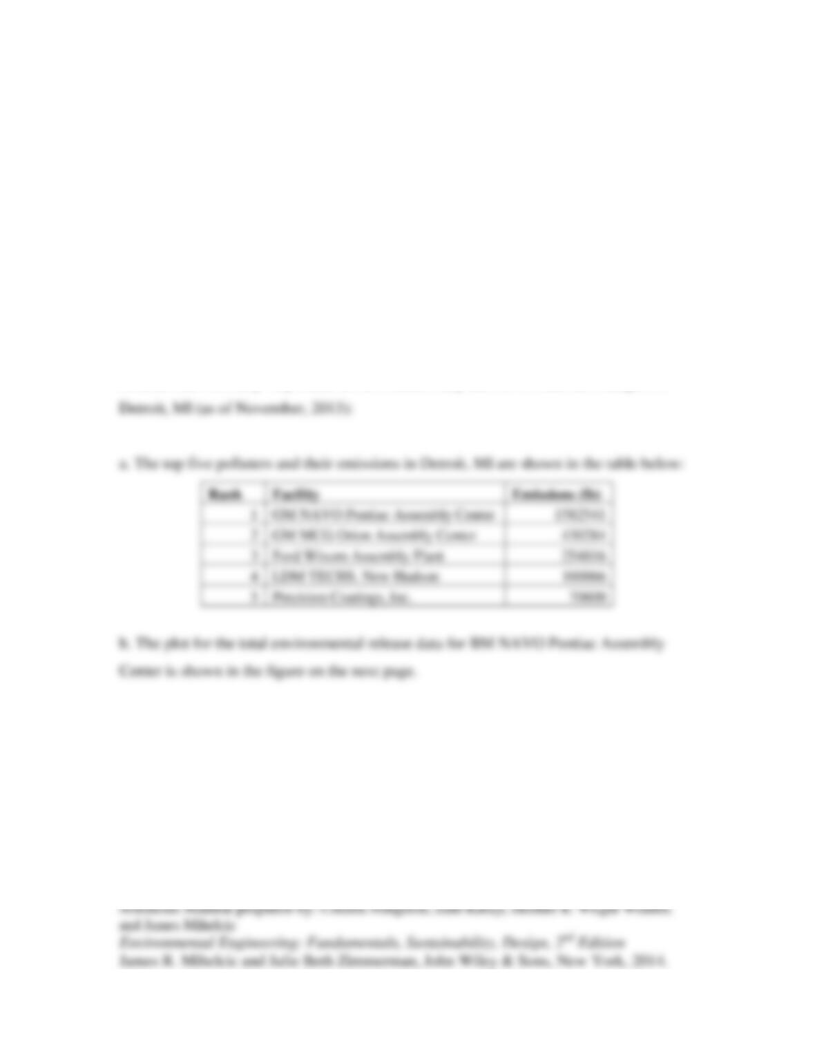
11.28 Investigate sources of hazardous air pollutants emitted near your community. Go to
Scorecard (www.scorecard.org) to gather data about air pollutant emissions. The
Scorecard site makes the Toxics Release Inventory easily searchable; by entering your
zip code, you can find a list of major air polluters in your area. (a) For your area, identify
the top three five polluters and their total emissions. (b) Plot total environmental release
for data from the top emitting company over the years of available data. (c) Describe the
overall trend of emissions over time.
Solution:
Students answers may vary based on the location they choose but here an example for
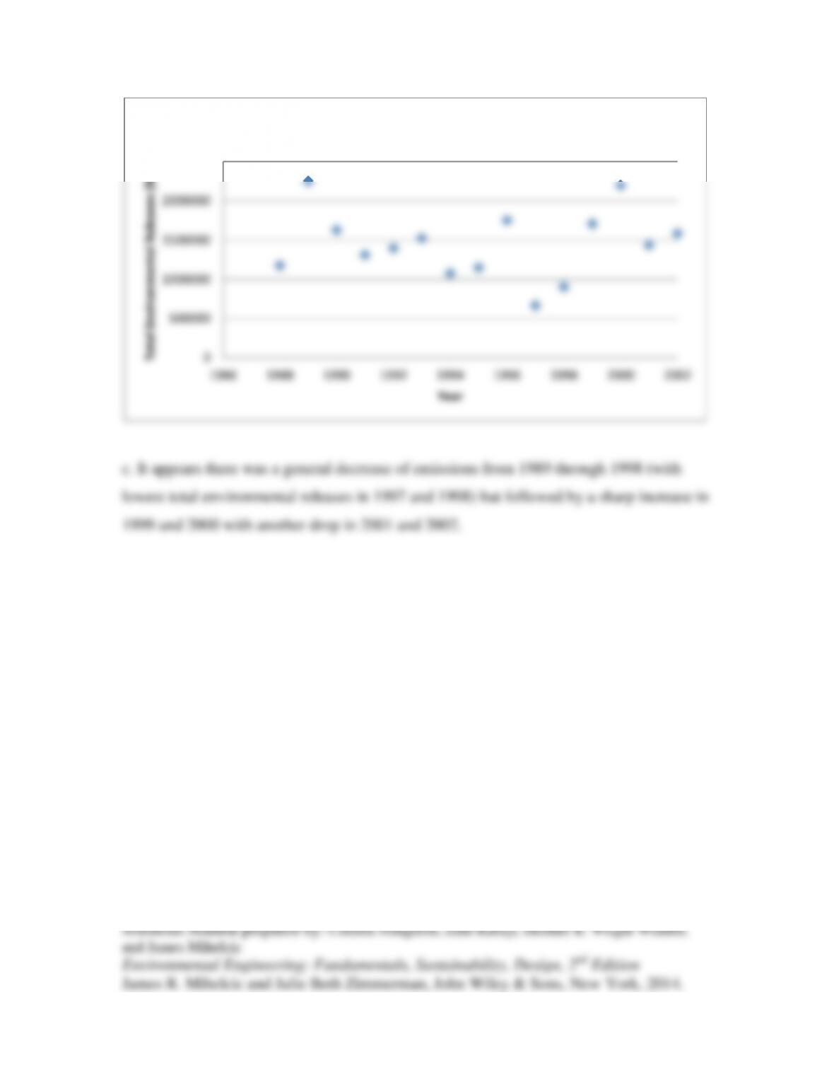
0
500000
1000000
1500000
2000000
2500000
Total Environmental Releases (lbs)
Total Environmental Releases over time for GM NAVO Pontiac Assembly
Center
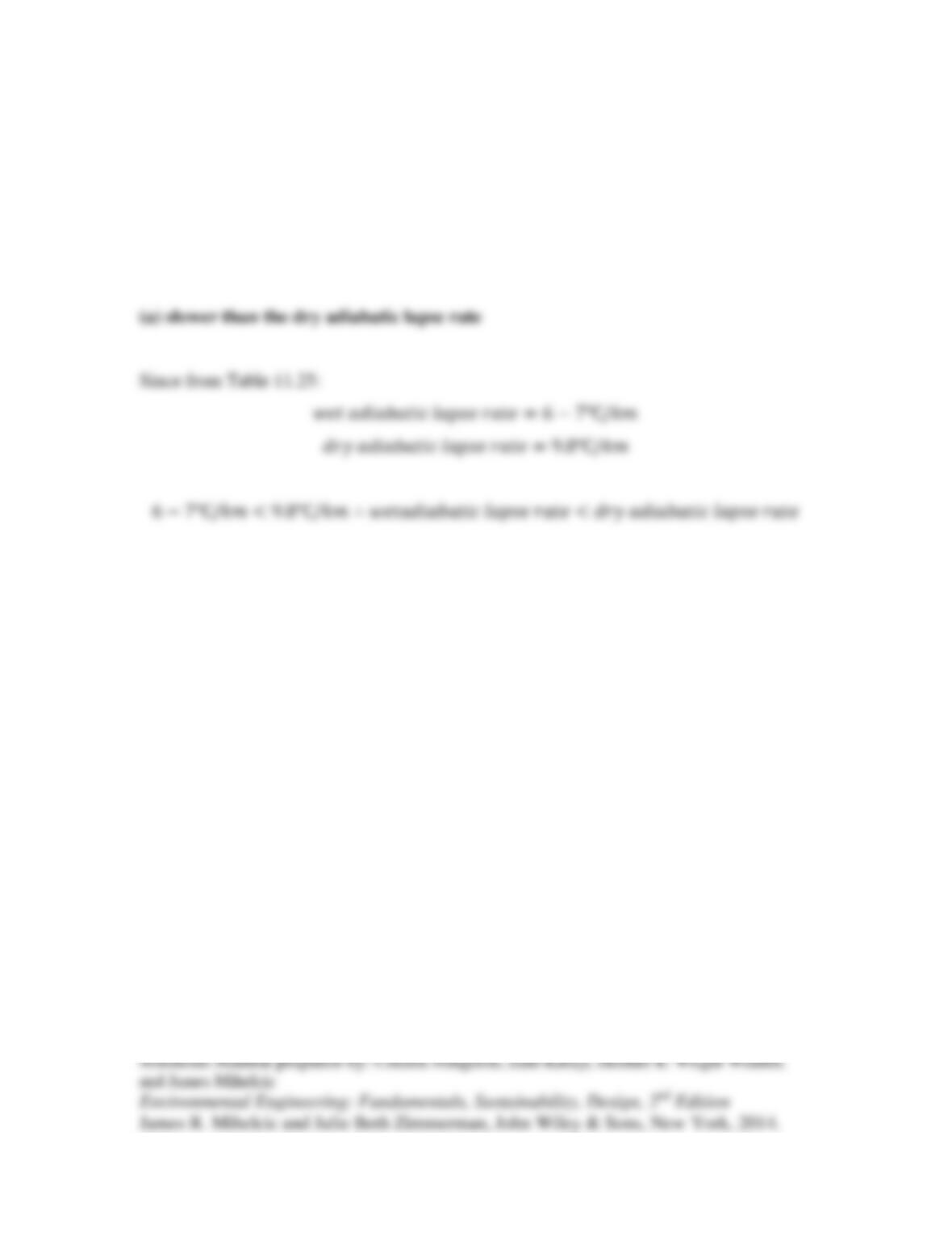
11.29 At the wet adiabatic lapse rate, the cooling rate of the air parcel is usually: (a)
slower than the dry adiabatic lapse rate, (b) the same as the dry adiabatic lapse rate, or,
(c) faster than the dry adiabatic lapse rate?
Solution:
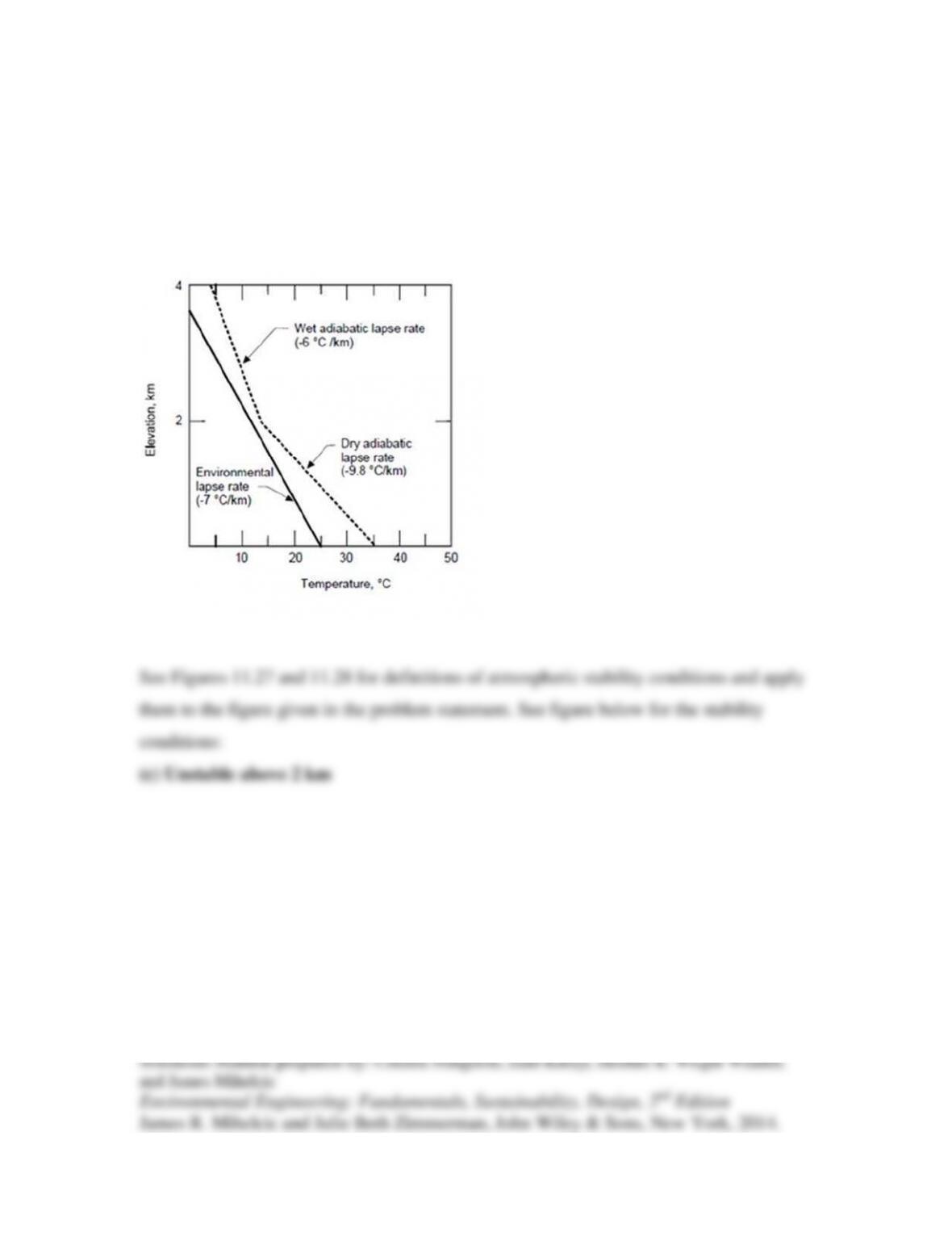
11.30 In the following figure, an air parcel is displaced and becomes saturated at an
elevation of 2 km. Which of the following stability conditions does the diagram depict?
(a) stable only below 1 km, (b) stable only above 1 km, (c) unstable above 2 km?
(problem from EPA, 2012h).
Solution:
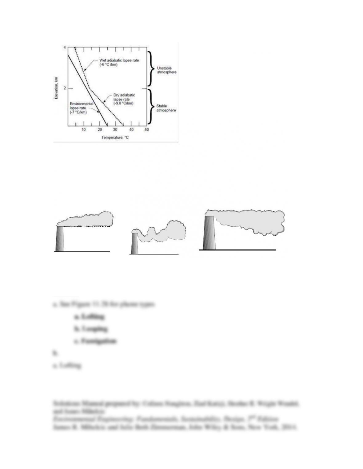
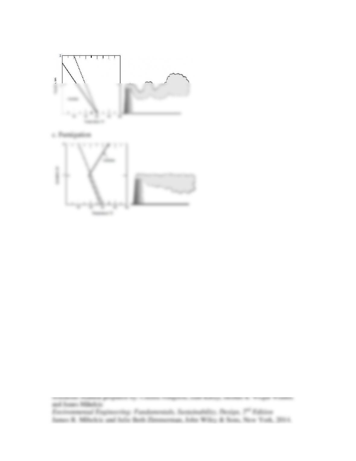
11.31 (a) Name the following three plume types. (b) sketch a graph of elevation on the y–
axis and air temperature on the x–axis that would describe the environmental lapse rate
and the lapse rate of an air parcel being emitted from the stack for each of these three
plume types.
a. b. c.
Solution:
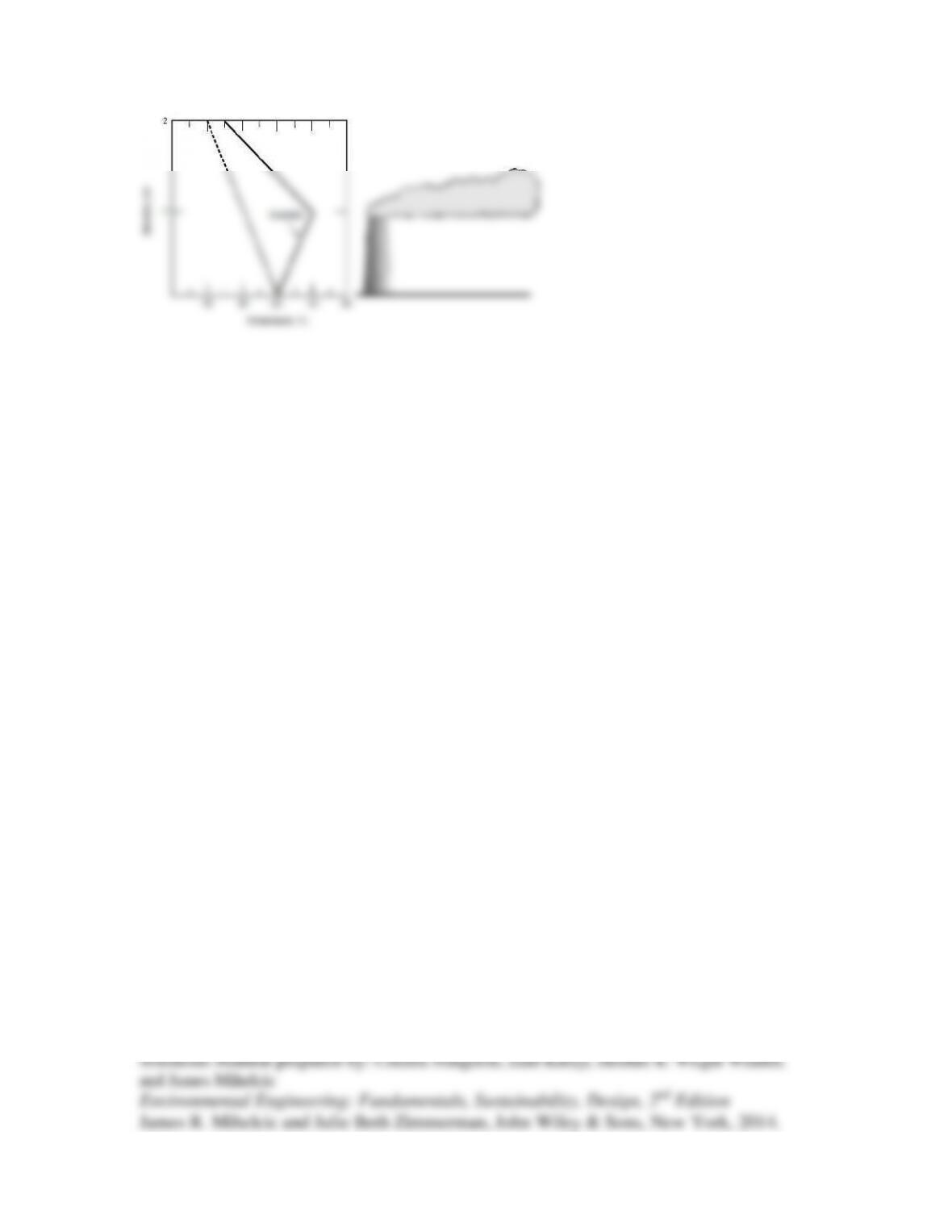
b. Looping
11.32 A fanning plume will occur when atmospheric conditions are generally (a) stable,
(b) highly unstable, or, (c) neutral?
Solution:
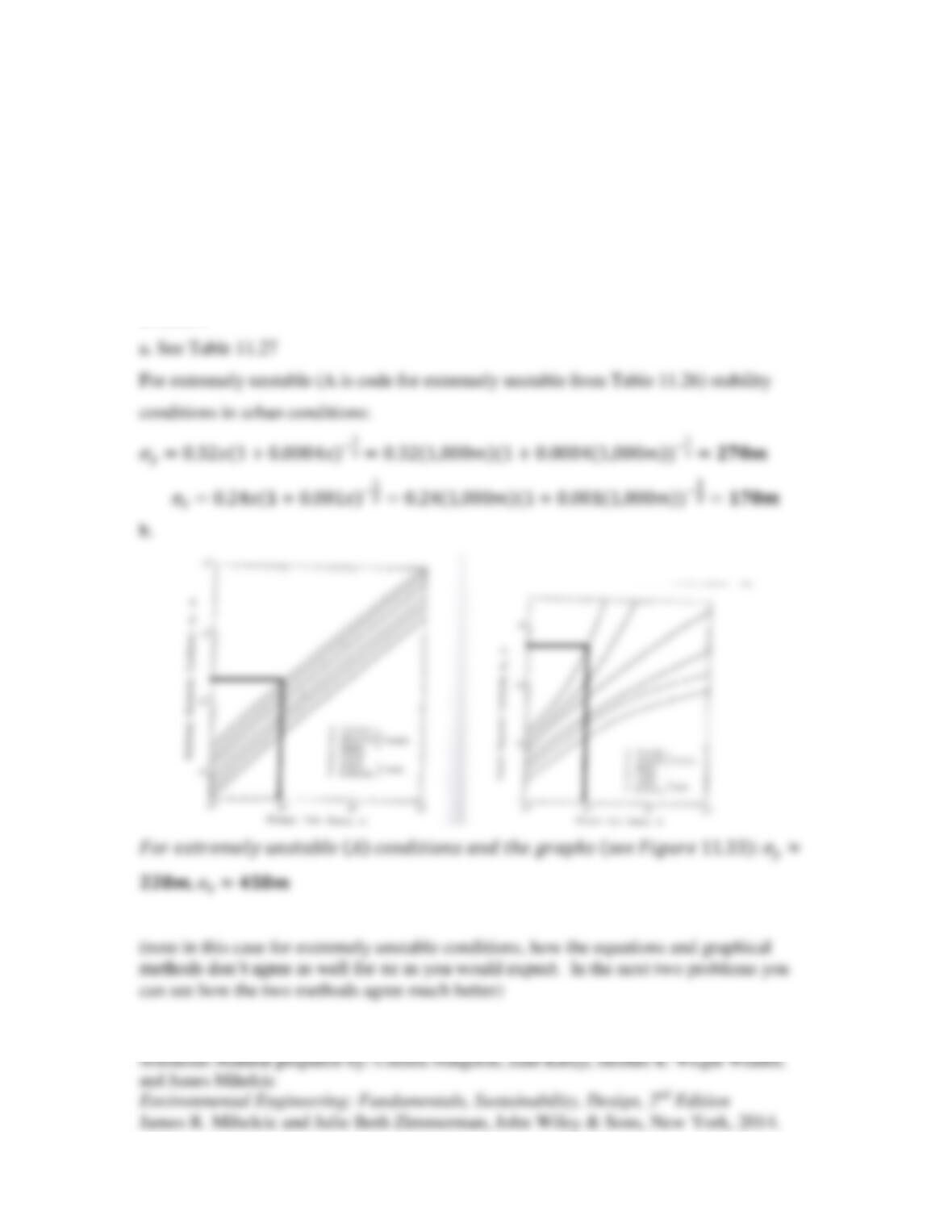
11.33 For extremely unstable atmospheric stability conditions, what are values for the
dispersion coefficient in the y and z directions 1,000 meters downstream in an urban area
from the point of the pollutant release? Estimate your values using two methods, (a) the
correct Briggs equation, and (b) a graphical method that allows you to estimate the
dispersion coefficients from established figures.
Solution:
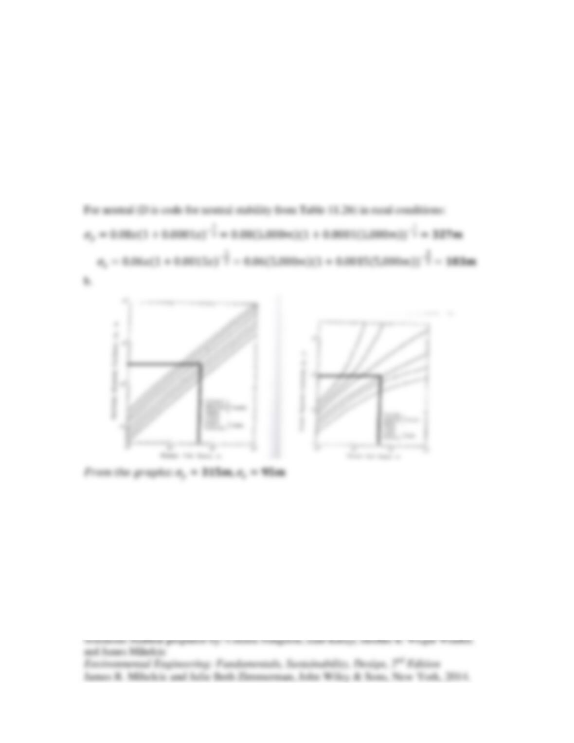
11.34 For neutral atmospheric stability conditions, what are values for the dispersion
coefficient in the y and z directions 5 km meters downstream in a rural area from the
point of the pollutant release? Estimate your values using two methods, (a) the correct
Briggs equation, and (b) a graphical method that allows you to estimate the dispersion
coefficients from established figures.
Solution:
a. See Table 11.27