
CHAPTER 15
AGGREGATE DEMAND AND AGGREGATE SUPPLY
MASTERY GOALS
The objectives of this chapter are to:
1. Use an aggregate demand (AD) curve to illustrate how price level changes affect
equilibrium GDP.
2. List the variables that cause the AD curve to shi! and explain their effects.
3. Use an aggregate supply (AS) curve to illustrate how a change in output affects the price
level in the short run, through its impact on unit costs.
4. Explain why, when the AS curve is derived, the nominal wage rate is assumed to be fixed.
5. List the variables that cause the AS curve to shi!, and explain their effects.
6. Use an AD–AS diagram to show how an economy arrives at a point of short-run
equilibrium.
7. Explain why the long-run AS curve is ver.cal.
8. Describe the economy’s self-correc.ng mechanism.
9. Explain how demand shocks affect the economy in the short run and in the long run.
10. Explain how supply shocks affect the economy in the short run and in the long run.
11. De(ne stag4a.on.
12. Summarize the issues that complicate the long-run adjustment process in the real world.
THE CHAPTER IN A NUTSHELL
This chapter shows that we can improve our understanding of economic 4uctua.ons by building
a model that allows for changes in the price level. The rela.onship between the price level and
output is a two-way rela.onship. Changes in the price level cause changes in real GDP, but
changes in real GDP also cause changes in the price level. The aggregate demand (AD) curve
illustrates the first causal rela.onship, while the aggregate supply (AS) curve illustrates the
second.
The AD curve tells us the equilibrium real GDP at any price level. This is the level of output at
which total spending equals total output. Movements along the AD curve occur when the price
level changes. The AD curve shi!s when anything other than a change in the price level causes
equilibrium GDP to change. These other influence include changes in government purchases,
autonomous consump.on spending, investment spending, net exports, taxes, and the money
supply.
The AS curve tells us the price level consistent with (rms’ unit costs and their percentage
markup at any level of output over the short run. Movements along the AS curve occur when a
change in total output causes a change in the price level. A change in output affects unit costs
and the price level in three key ways: it will cause a change in nonlabor input prices, it will cause
a change in input requirements per unit of output, and it will cause a change in the nominal
wage. Since nominal wages respond slowly to changes in output, the AS curve is derived while
assuming that the nominal wage rate is given.
The AS curve shi!s when anything other than a change in real GDP causes the price level to
change. Short-run changes in unit costs that are not caused by changes in output (such as
changes in world oil prices or the weather) and changes in nominal wage rates cause the AS
curve to shi!. Unit costs change in the short run because of changes in world oil prices, the
weather, technology, and the nominal wage. (A later sec.on of the chapter examines a change
in the nominal wage.)
Short-run equilibrium is at the intersec.on of the AD and AS curves.
A demand shock is an event that causes the AD curve to shi!. A posi.ve demand shock shi!s
the AD curve to the right and increases both real GDP and the price level in the short run. A
nega.ve demand shock shi!s the AD curve to the le! and decreases both real GDP and the
price level in the short run.
When a demand shock pulls the economy away from full employment, changes in the wage rate
will shi! the AS curve, eventually causing the economy to self-correct and return to
full-employment output. A ver.cal long-run AS curve illustrates this result. This long-run AS
curve shows that the economy behaves as the classical model predicts a!er the self-correc.ng
mechanism has done its job. Demand shocks cannot change equilibrium GDP in the long run. An
increase in government purchases, for instance, causes a complete crowding out effect that
leaves total output and total spending unchanged. Since it can take several years to return the
economy to full-employment a!er a demand shock, governments are reluctant to rely on the
self-correc.ng mechanism alone to keep the economy on track, and rely on (scal and monetary
policies to return to full-employment more quickly.
A supply shock is an event that causes the AS curve to shi!. A nega.ve supply shock shi!s the
AS curve upward, causing stag4a.on in the short run, while a posi.ve supply shock shi!s the AS
curve downward, increasing output and decreasing the price level. In the long run, however,
supply shocks self-correct in the same way as demand shocks, so that the economy returns to
full employment.
In the real world, several things complicate the adjustment process as described in the chapter.
To draw the AS curve, this chapter assumes that output prices are completely 4exible in the
short run, and that nominal wages are completely rigid in the short run. But in some markets,

output prices are not completely 4exible, and nominal wages are not completely rigid, in the
short run. In addi.on, recovering from a demand or supply shock requires adjustments other
than changes in prices and wages. While these observa.ons complicate the adjustment process
in the real world, they do not change the basic outlines of that process as described in the
chapter.
The AD and AS curves are tools that help us understand important economic events. This
chapter closes by using these tools to explain the forces behind the recessions of 1990–91 and
2008-2009.
DEFINITIONS
In order presented in chapter.
Aggregate demand (AD) curve: A curve indica.ng equilibrium GDP at each price level
when the money supply is constant.
Aggregate supply (AS) curve: A curve indica.ng the price level that is consistent with
(rms’ unit costs and markups for any level of output over the short run.
Short-run macroeconomic equilibrium: A combina.on of price level and GDP
consistent with both the AD and AS curves.
Demand shock: Any event that causes the AD curve to shi!.
Supply shock: Any event that causes the AS curve to shi!.
Self-correcting mechanism: The adjustment process through which price and wage
changes return the economy to full-employment output in the long-run.
Long-run aggregate supply curve: A ver.cal line indica.ng all possible output and
price-level combina.ons at which the economy could end up in the long run.
Stag ation: The combina.on of falling output and rising prices.
TEACHING TIPS
1. It’s easy for students to lose sight of the main point that the chapter makes (i.e., that the
price level and the equilibrium level of GDP are determined simultaneously) as they
work through its details. Repeated reminders of this joint determina.on are in order.
2. Stress that changes in the money market will have different effects on the AD curve,
depending on the origin of the money market change.
a. A change in the price level (which shi!s the money demand curve) will lead to a
movement along the exis.ng AD curve.

b. A change in the money supply or a change in preferences concerning money demand
(which shi!s the money demand curve) will lead to a shi! of the en.re AD curve.
3. Have students trace the effects on the AD curve of the autonomous increase in money
demand that occurred in 1980–81. This will help clarify the sources of shi!s in AD
curves, as well as show the overall macroeconomic effects of this shock. A good
reference is the paper by William Poole, “Monetary Policy Lessons of Recent In4a.on
and Disin4a.on,” Journal of Economic Perspectives, Summer, 1988. He discusses the
macroeconomic impact of the increase in money demand due to financial innova.ons.
DISCUSSION STARTERS
1. Remind students that money demand rises when the price level rises because people
will need more money to make their everyday purchases. In the example in the chapter,
the price index rose from 100 to 140. Use this increase to calculate how many extra
dollars an individual will need to buy the following:
a. Fi!een gallons of gas that ini.ally sold for $1.24 per gallon.
b. An apartment that originally rented for $900 per month.
c. A movie .cket that ini.ally cost $7.
A second way to show that changes in the price level lead to changes in money demand
is to have students keep track of their personal expenditures for one day and then
calculate how much more expensive these purchases would be if the price index rose
from 100 to 140. Remind them that when the general price level rises, they cannot
subs.tute toward rela.vely cheaper goods.
2. For each of the four following graphs, have students:
a. Explain why the economy is not in short-run macroeconomic equilibrium at the point
indicated.
b. Describe the adjustment process that will move the economy to short-run
macroeconomic equilibrium.
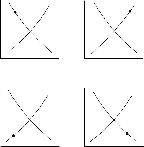
A
AS
AD
AS
AD
B
C
AS
AD
D
AS
AD
3. Students can become confused when they learn that (scal and monetary policies are
ineffec.ve in the long run. This is not the same as saying the economy will always return
to its star.ng point a!er a (scal or monetary change. Whether that occurs depends on
where the economy is when the shock occurs.
a. Draw an AD–AS graph with a short-run equilibrium below the full-employment level
of output. Ask students to show either the effect of an increase in the money supply
or the effect of an increase in government spending that is suGciently large to move
the economy to equilibrium at full-employment. Ask them if the economy will move
back to the ini.al short-run equilibrium point. (It won’t.)
b. Draw an AD–AS graph with a short-run equilibrium at the full-employment level of
output. Again, ask them to show either the effect of an increase in the money supply
or the effect of an increase in government spending that moves the economy to a
new equilibrium. Ask them if the economy will move back to its ini.al equilibrium. (It
will.)
c. Compare the outcomes in parts (a) and (b) to show that monetary and (scal policies
will have permanent effects on the economy if the economy is not at
full-employment, but will not have permanent effects if the economy is at
full-employment. Discuss the costs and benefit of using monetary or (scal policy to
move the economy to a point where it was already headed.
4. Show students evidence of labor market disequilibrium where shortages lead to wage
increases that may affect the economy’s in4a.on rate. One possibility would be the
June, 1997, managerial and professional unemployment rate of 2%. (See Michael Hirsh,
“Begging for Bosses,” Newsweek, July 14, 1997.) Ask students if they “see” this low
unemployment rate as a signal for entry into managerial and professional occupa.ons.
How do they plan to respond to this signal? (Some may want to be managers already,
some may plan to change their career plans, and some may con.nue on whatever career
path they already have.) Can they respond to this signal by entering the market
immediately? What training is necessary before they could enter this market? Discuss
who will respond to this signal in the short run and who will respond to this signal in the
long run.