
CHAPTER 11
THE SHORT-RUN MACRO MODEL
MASTERY GOALS
The objectives of this chapter are to:
1. Explain the usefulness of the short-run macro model.
2. List the four components of aggregate expenditure included in the simple macro model of
this chapter.
3. List the determinants of consumption spending and describe their effects on consumption
spending.
4. Describe a consumption function in terms of autonomous consumption and the marginal
propensity to consume.
5. Show how changes in taxes and in autonomous consumption changes affect the
consumption-income line.
6. Explain why inventory investment is not included in aggregate expenditure.
7. Define government spending.
8. Define net exports.
9. Explain why investment, government spending, and net exports are assumed to be
determined by forces outside the short-run macro model.
10. Use a 45 translator line, together with the aggregate expenditure line, to show inventory
changes and to find the short-run equilibrium output level.
11. Explain why short-run equilibrium output is not necessarily full-employment output.
12. Use the multiplier to show how a change in spending affects equilibrium output in an
economy.
13. Give examples of automatic stabilizers/destabilizers and explain how they
reduce/increase the impact of changes in spending.
14. Discuss the size of multiplier in the real-world.
15. Use the short-run macro model of the chapter to explain the causes of the 2008–09
recession.
THE CHAPTER IN A NUTSHELL
The main purpose in building the short-run macro model is to explain fluctuations in real GDP
that the long-run, classical model cannot explain. The short-run macro model focuses on the role
of spending in explaining economic fluctuations. It explains how shocks that initially affect one
sector of the economy quickly influence other sectors, causing changes in total output and
employment. In this chapter, spending is the only force that determines how much output the
economy will produce.
The short-run macro model focuses on spending in markets for currently produced U.S. goods
and services—that is, spending on things that are included in U.S. GDP. Spending has four
components: (real) consumption spending, (real) investment spending, (real) government
purchases, and (real) net exports.
Consumption is positively related to real disposable income, real wealth, and expectations of
future income, and is negatively related to the interest rate.
The consumption function illustrates the relationship between consumption and disposable
income. Changes in disposable income lead to movements along the consumption function. The
slope of the consumption function is equal to the marginal propensity to consume, that is, the
amount by which consumption spending changes when disposable income rises by one dollar.
The vertical intercept represents autonomous consumption spending, the combined impact on
consumption spending of everything other than disposable income. Changes in wealth, the
interest rate, or expectations of future income lead to a change in autonomous consumption
spending. These changes are shown graphically as a shift of the consumption schedule.
The consumption-income line shows the relationship between real consumption spending and
real income, rather than real disposable income. When the government collects a fixed amount of
taxes from households, the consumption-income line shifts downward by the amount of the tax
times the MPC. The slope of the consumption-income line, however, is unaffected by taxes, and
is equal to the MPC.
A change in income causes consumption spending to change and leads to a movement along the
consumption-income line, while consumption spending changes that occur for any other reason
will cause the consumption-income line to shift. These other changes work by changing
autonomous consumption or taxes.
In the short-run macro model, (planned) investment spending includes plant and equipment
purchases by business firms, and new home construction. Inventory investment is treated as
unintentional and undesired, and is therefore excluded from the definition. Government
purchases include all of the goods and services that government agencies buy during the year.
Net exports equal exports minus imports. Export spending measures production sold to
foreigners, while import spending measures our spending on foreign output. Thus, to accurately
measure domestic output, we must add U.S. exports and subtract U.S. imports. These two
adjustments can be made together by simply including net exports as the foreign sector’s
contribution to total spending. Investment spending, government purchases, and net exports are
all treated as given values, determined by forces outside of this model.
Aggregate expenditure (AE) is the sum of spending by households, businesses, the government,
and the foreign sector on final goods and services. Since the relationship between income and
spending is circular, when income increases, aggregate expenditure will rise by the MPC times
the change in income.
When aggregate expenditure is less than GDP, output will decline in the future. Similarly, when
aggregate expenditure is greater than GDP, output will tend to rise in the future. Therefore, in the
short run, equilibrium GDP is the level of output where output and aggregate expenditure are
equal.
Output minus aggregate expenditures equals the change in inventories during any period. When
output equals aggregate expenditures, then inventory changes will equal zero, so another way to
find the equilibrium GDP in the economy is to find the output level where inventory changes are
equal to zero.
Graphically, equilibrium GDP is found at the intersection of the aggregate expenditure line and
the 45 line. At any output level where the aggregate expenditure line lies below the 45 line,
aggregate expenditure is less than GDP and inventory accumulation will cause firms to reduce
output in the future. At any output level where the aggregate expenditure line lies above the 45
line, aggregate expenditure is greater than GDP and inventory depletion will cause firms to
increase output in the future.
Operating at equilibrium does not guarantee full employment. If aggregate spending is too high
or too low, the aggregate expenditure line will cross the 45 line at some output level other than
full employment output, and the economy will remain at a short-run equilibrium where full
employment is not achieved.
Changes in spending—in investment, government purchases, or autonomous consumption—lead
to a multiplier effect on GDP, where the initial shock sets off a chain reaction, leading to
successive rounds of changes in spending and income. The expenditure multiplier is the number
by which the initial spending change is multiplied to get the change in equilibrium GDP. The
formula for the expenditure multiplier is 1/(1 – MPC).
Automatic stabilizers reduce the size of the multiplier, and therefore reduce the impact of
spending changes. They work by shrinking the additional spending that occurs in each round of
the multiplier. Some real-world automatic stabilizers are changes in taxes, transfer payments,
interest rates, imports, and forward-looking behavior. Perhaps the most important automatic
stabilizer of all is the passage of time—in the long run our multipliers have a value of zero. After
any change in spending, output will eventually return to full employment, so the change in
equilibrium GDP will be zero.
Automatic destabilizers increase the size of multiplier, and therefore increase the impact of
spending changes. They work by increasing the additional spending that occurs in each round of
the multiplier. Some real-world automatic destabilizers are asset prices and wealth, and
investment spending.
In the real world, the multiplier is impacted by both automatic stabilizers and automatic
destabilizers so coming a real value can be difficult. Economists generally agree that the current
number is smaller than it was during the Great Depression and most put the actual value in the
neighborhood of 1.5. In the long run, however, the value of the multiplier is zero.

The recession of 2008-09 was caused by a spike in oil prices and the collapse of the housing
bubble, as discussed in chapter 4. After the declines in spending fueled by the first two events,
the U.S. economy was hit by a third event: a serious financial crisis. All of these events caused
a significant decline in investment and consumption spending. Over time, as the multiplier
process took place, the decrease in spending brought down both GDP and employment.
There are two appendices to this chapter. The first explains how to use algebraic equations to
find equilibrium GDP, while the second explains the special case of the tax multiplier.
Short-run macro model: A macroeconomic model that explains how changes in spending
can affect real GDP in the short run.
Consumption function: A positively sloped relationship between real consumption
spending and real disposable income.
Autonomous consumption spending: The part of consumption spending that is
independent of income; also the vertical intercept of the consumption function.
Marginal propensity to consume: The amount by which consumption spending rises
when disposable income rises by one dollar.
Consumption-income line: A line showing aggregate consumption spending at each level
of income or GDP.
Aggregate expenditure (AE): The sum of spending by households, business firms, the
government, and foreigners on final goods and services produced in the United States.
Equilibrium GDP: In the short run, the level of output at which output and aggregate
expenditure are equal.
Expenditure multiplier: The amount by which equilibrium real GDP changes as a result of
a one-dollar change in autonomous consumption, investment spending, government purchases,
or net exports.
Automatic stabilizer: A feature of the economy that reduces the size of the expenditure
multiplier and diminishes the impact of spending changes on real GDP.
Automatic destabilizer: A feature of the economy that increases the size of the expenditure
multiplier and enlarges the impact of spending changes on real GDP.
1. Stress that, in the model of this chapter, firms want to keep output equal to sales, so that
inventory stocks won’t change. Thus, changes in inventories signal producers to increase
or decrease production. Explain that firms have optimal inventory levels. If actual
inventory falls below the optimal level, then firms risk not having merchandise on hand
to meet unpredictable peaks in demand. If actual inventory rises above the optimal level,
then firms incur excessive storage costs.
2. It is important to stress that investment spending (IP) is one of the spending aggregates
while actual investment (I) is a component of GDP. This means that while aggregate
expenditure is equal to the sum of C + IP + G NX, GDP is equal to the sum of C + I + G
NX. Emphasize to students that there is only one term that is different in these two
equations. Explain that, since this is the case, the only way that aggregate expenditures
can equal GDP is if IP is equal to I. This will help students see that in equilibrium,
investment spending and actual investment are equal.
DISCUSSION STARTERS
1. Have students look at the current state of the economy. (Refer to
hp://research.stlouisfed.org/fred/data/gdp/gdppot for potential real GDP !gures to
compare with actual real GDP numbers from www.bea.doc.gov/bea/dn/nipaweb ,
“Selected NIPA tables, table 1.2.” Refer to www.bls.gov for the unemployment rate and
changes in the CPI.) Discuss whether the economy appears to be at full employment. Do
they !nd con/icting evidence?
2. To emphasize the difference between the short-run macro model and the long-run
classical model, ask students how automobile manufacturers initially respond to an
overstock of cars. Some students may say that they offer rebates; point out that this
typically happens in slow markets but is not the first response. The first response is to lay
off workers until the glut disappears (they close the plant or reduce the number of shifts
for two weeks, or however long they deem necessary). Notice that the manufacturers do
not respond by cutting wages and car prices. Explain that this unemployment is predicted
by the short-run macro model, but is not predicted by the long-run classical model.
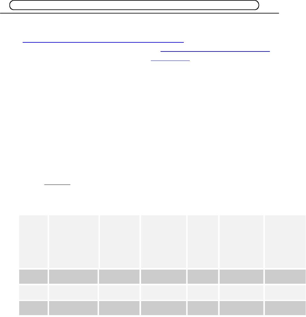
3. Recall the results from Table 4 in the chapter: when investment spending was equal to
$800 billion, the equilibrium GDP was $8,000 billion. Examine the effect of a $400
billion decrease in planned investment by reworking columns 3, 6, and 7 of the table, and
using the results to find the new equilibrium level of GDP. Check your results by using
the multiplier.
Answer:
(1)
Incom
e or
GDP
(2)
Consumptio
n Spending
(3)
Investme
nt
Spending
(4)
Governme
nt
Spending
(5)
Net
Export
s
(6)
Aggregate
Expenditur
e
(7)
Change
in
Inventori
es
4,000 3,200 400 1000 600 5,200 –1,200
5,000 3,800 400 1000 600 5,800 –800
6,000 4,400 400 1000 600 6,400 –400
7,00
0
5,000 400 1000 600 7,000 0
8,000 5,600 400 1000 600 7,600 400
9,000 6,200 400 1000 600 8,200 800
10,00
0
6,800 400 1000 600 8,800 1200
11,00
0
7,400 400 1000 600 9,400 1600
12,00
0
8,000 400 1000 600 10,000 2000
GDP = multiplier aggregate expenditure
GDP = 2.5 –$400 = –$1,000
The new equilibrium GDP = the original equilibrium GDP level + GDP
The new equilibrium GDP = $8,000 + –$1,000 = $7,000
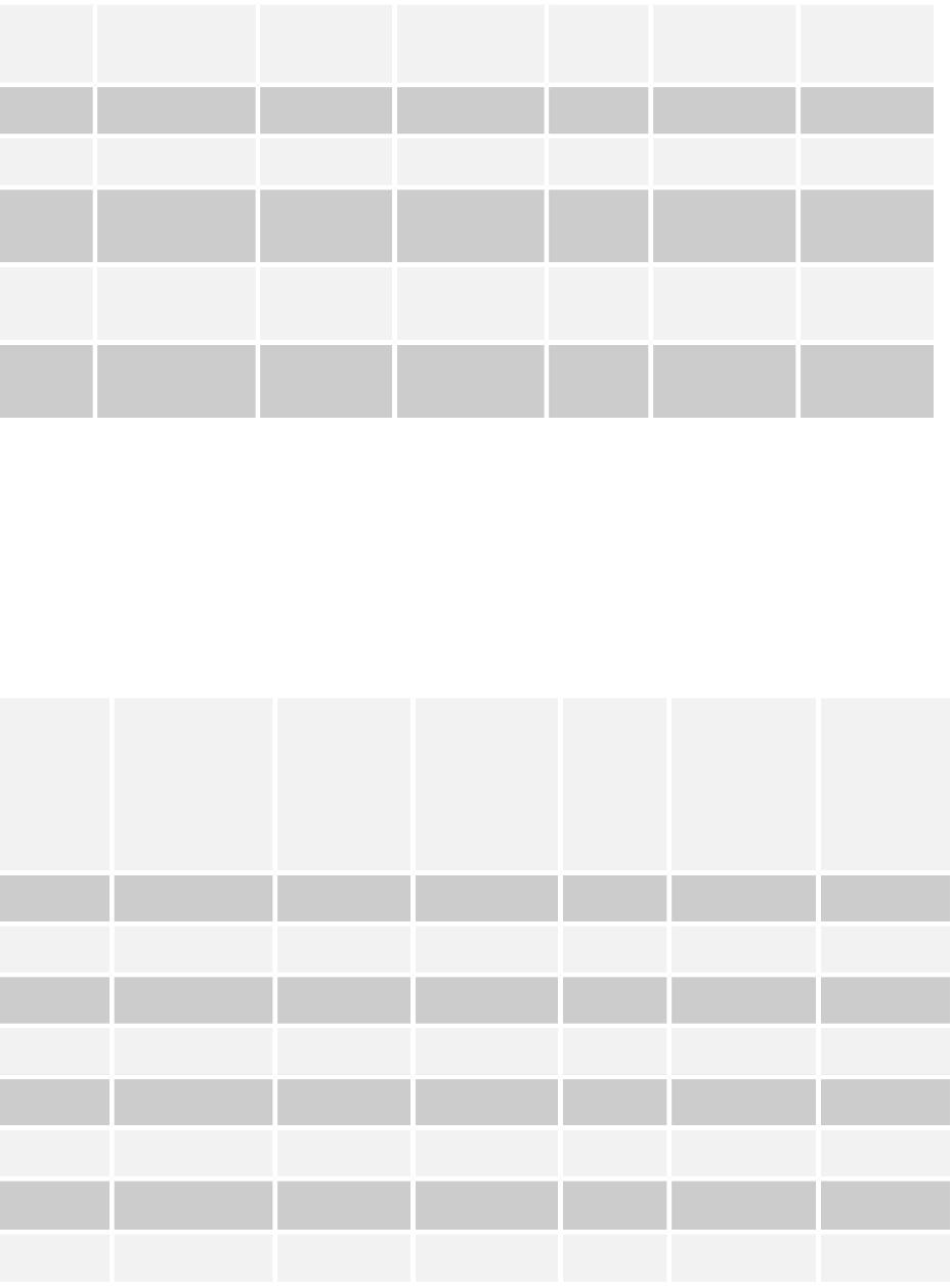
5. Once again, use Table 4 to explore a change in spending—this time, an $800 billion
increase in government spending—by reworking columns 4, 5, and 6. Find the new
equilibrium GDP, and check your results by using the multiplier.
Answer:
(1)
Income
or GDP
(2)
Consumptio
n Spending
(3)
Investme
nt
Spending
(4)
Governme
nt
Spending
(5)
Net
Exports
(6)
Aggregate
Expenditur
e
(7)
Change
in
Inventori
es
4,000 3,200 800 1,800 600 6,400 –2,400
5,000 3,800 800 1,800 600 7,000 –2,000
6,000 4,400 800 1,800 600 7,600 –1,600
7,000 5,000 800 1,800 600 8,200 –1,200
8,000 5,600 800 1,800 600 8,800 –800
9,000 6,200 800 1,800 600 9,400 – 400
10,000 6,800 800 1,800 600 10,000 0
11,000 7,400 800 1,800 600 10,600 400

12,000 8,000 800 1,800 600 11,200 800
GDP = multiplier X aggregate expenditure
GDP = 2.5 $800 = $2,000
The new equilibrium GDP = the original equilibrium GDP level + GDP
The new equilibrium GDP = $8,000 + $2,000 = $10,000