
Supplement
D Linear Programming
1. Characteristics of Linear Programming Models
1. Linear programming is an optimization process with several characteristics
a. A single objective function states mathematically what is being maximized or minimized.
b. Decision variables represent choices that the decision maker can control. Solving the
problem yields their optimal values based on the assumption that decision variables are
continuous.
c. Constraints are limitations that restrict the permissible choices for the decision variables,
which can be expressed mathematically in one of three ways:
d. The feasible region includes all permissible combinations of the decision variables which
satisfy the given constraints. Usually an infinite number of possible solutions.
e. A parameter, also known as a coefficient or given constant, is a value that the decision
maker cannot control and that does not change when the solution is implemented.
• Assume parameters are known with certainty, and without doubt.
f. The objective function and constraints are assumed to be linear, which implies
proportionality and additivity—there can be no products or powers of decision variables.
g. We assume the model to exhibit nonnegativity, which means that the decision variables
must be positive or zero.
2. Formulating a Linear Programming Model
1. Step 1: Define the decision variables.
a. What must be decided?
b. Define each decision variable specifically, remembering that the definitions must be
equally useful in the constraints.
2. Step 2: Write out the objective function.
a. What is to be maximized or minimized?
b. Write out an objective function to make what is being optimized a linear function of the
decision variables.
3. Step 3: Write out the constraints.
a. What limits the values of the decision variables?

b. Identify the constraints and the parameters for each decision variable in them. To be
formally correct, also write out the nonnegativity constraints.
c. As a consistency check, make sure the same unit of measure is being used on both sides
of each constraint and the objective function.
4. Problem Formulation. Use Application D.1: Crandon Manufacturing.
The Crandon Manufacturing Company produces two principal product lines. One is a
portable circular saw, and the other is a precision table saw. Two basic operations are
crucial to the output of these saws: fabrication and assembly. The maximum fabrication
capacity is 4000 hours per month; each circular saw requires 2 hours, and each table saw
requires 1 hour. The maximum assembly capacity is 5000 hours per month; each circular
saw requires 1 hour, and each table saw requires 2 hours. The marketing department
estimates that the maximum market demand next year is 3500 saws per month for both
products. The average contribution to profits and overhead is $900 for each circular saw
and $600 for each table saw.
Management wants to determine the best product mix for the next year to maximize
contribution to profits and overhead. Also, it is interested in the payoff of expanding
capacity or increasing market share.
Definition of Decision Variables
1
x
= number of circular saws produced and sold per month
2
x
= number of table saws produced and sold per month
Formulation
Maximize:
Zxx =+ 21 600900
Subject to:
( )
( )
( )
( )
ityNonnegativxx
Demandxx
Assemblyxx
nFabricatioxx
0,
500,311
000,521
000,412
21
21
21
21
+
+
+
3. Graphic Analysis
1. The purpose is to gain insight into the meaning of the computer output by analyzing a simple
two-variable problem.
2. Five basic steps
a. Plot the constraints
• Active Model D.1 in MyLab Operations Management offers many insights on
graphic analysis. Use it when studying examples D.2 through D.4.
• Tutor D.1 in MyLab Operations Management provides a new practice example for
plotting the constraints.
b. Identify the feasible region
• The feasible region is the area on the graph that contains the solutions which satisfy
all of the constraints simultaneously, including the nonnegativity restrictions.
• Locate the area that satisfies each of the constraints.
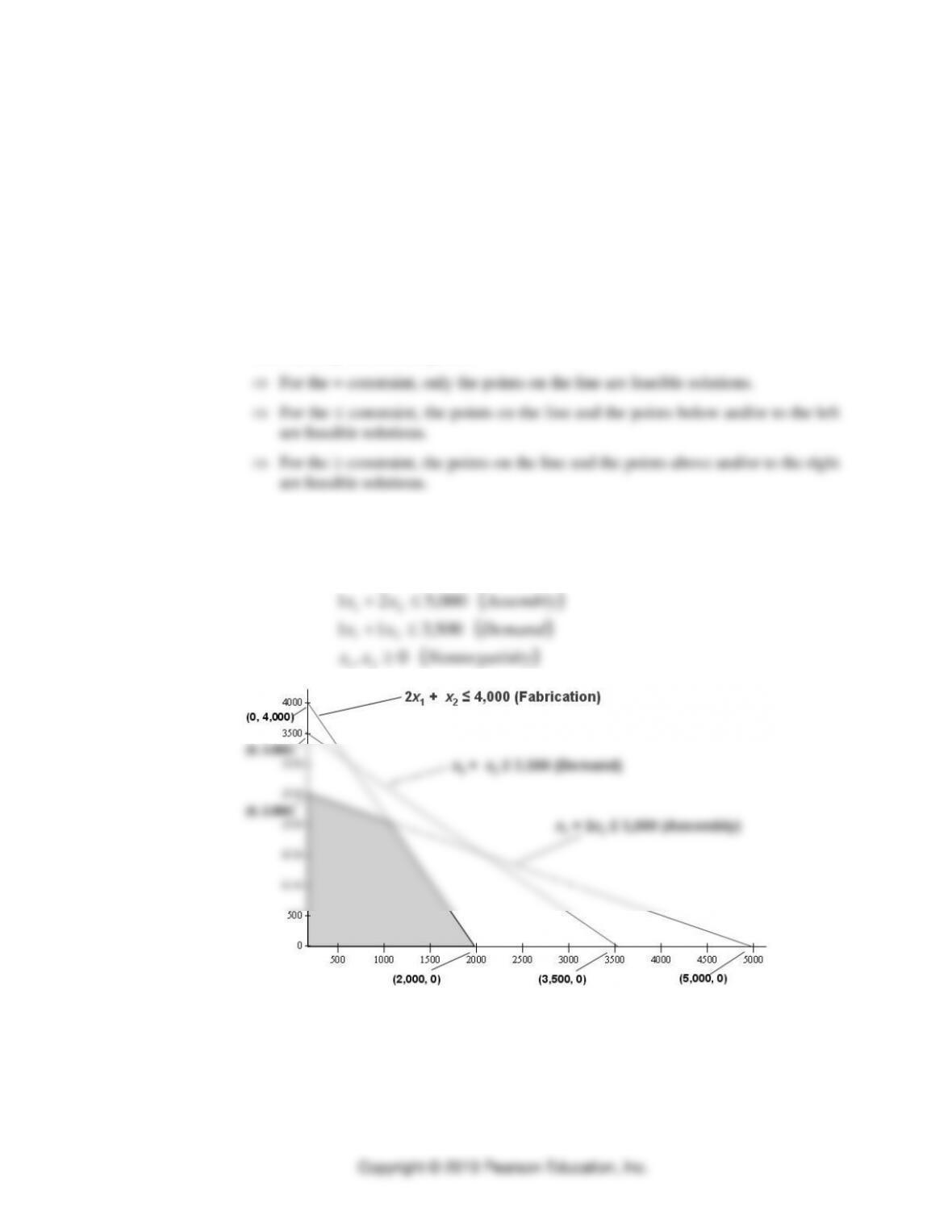
• Locate the area that satisfies all of the constraints. Generally, the following three
rules identify the feasible points:
• Use Application D.2: Steps a and b for Crandon Manufacturing.
Plot constraint equations
( )
( )
( )
( )
ityNonnegativxx
Demandxx
Assemblyxx
nFabricatioxx
0,
500,311
000,521
000,412
21
21
21
21
+
+
+
Copyright © 2019 Pearson Education, Inc.
Point 1
Point 2
Constraint
x1
x2
x1
x2
1
0
4,000
2,000
0
2
0
2,500
5,000
0
3
0
3,500
3,500
0
Shade feasible region
c. Plot an objective function line
• Limit search for solution to the corner points.
• A corner point lies at the intersection of two (or possibly more) constraint lines on the
boundary of the feasible region.
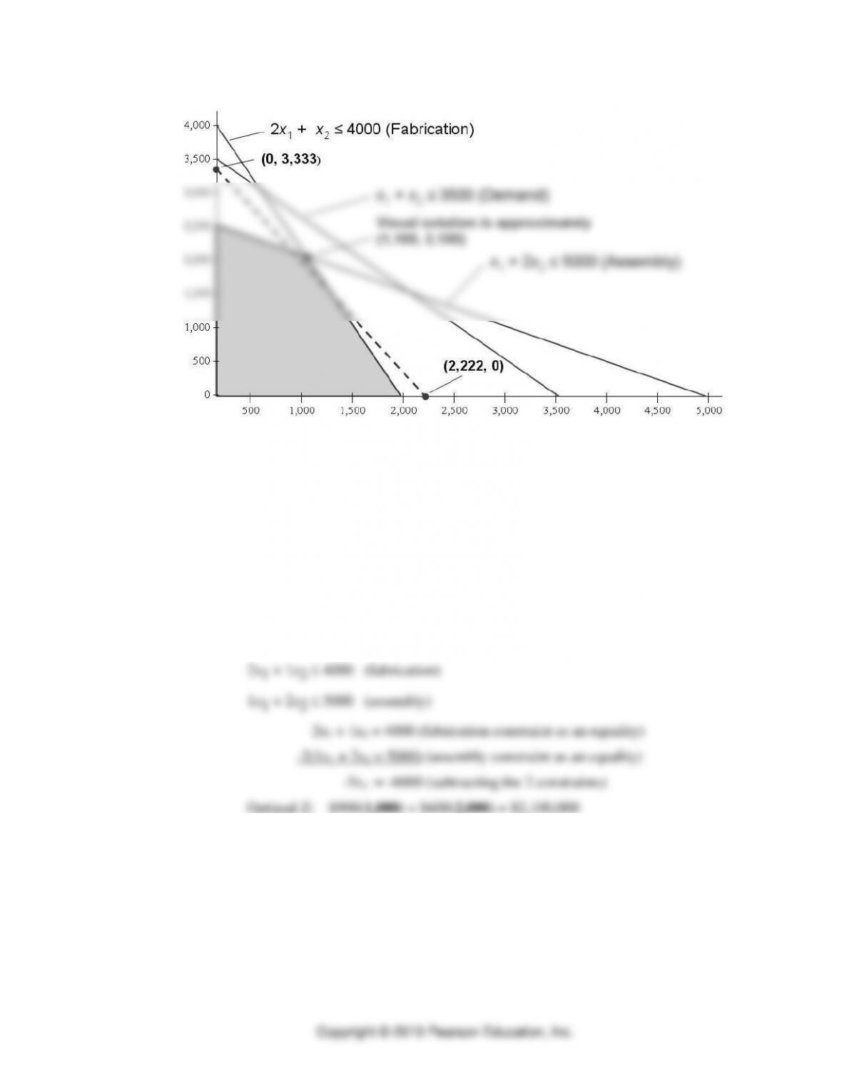
d. Find the visual solution
• For maximization problems, the best solution is a point on the iso-profit line farthest
from the origin. For minimization problems, the best solution is a point on the iso-
cost line closest to the origin.
• Use Application D.3: Steps c and d for Crandon Manufacturing.
Plot iso-profit lines and identify the visual solution
Let Z = $2,000,000 (arbitrary choice)
Plot $900x1 + $600x2 = $2,000,000
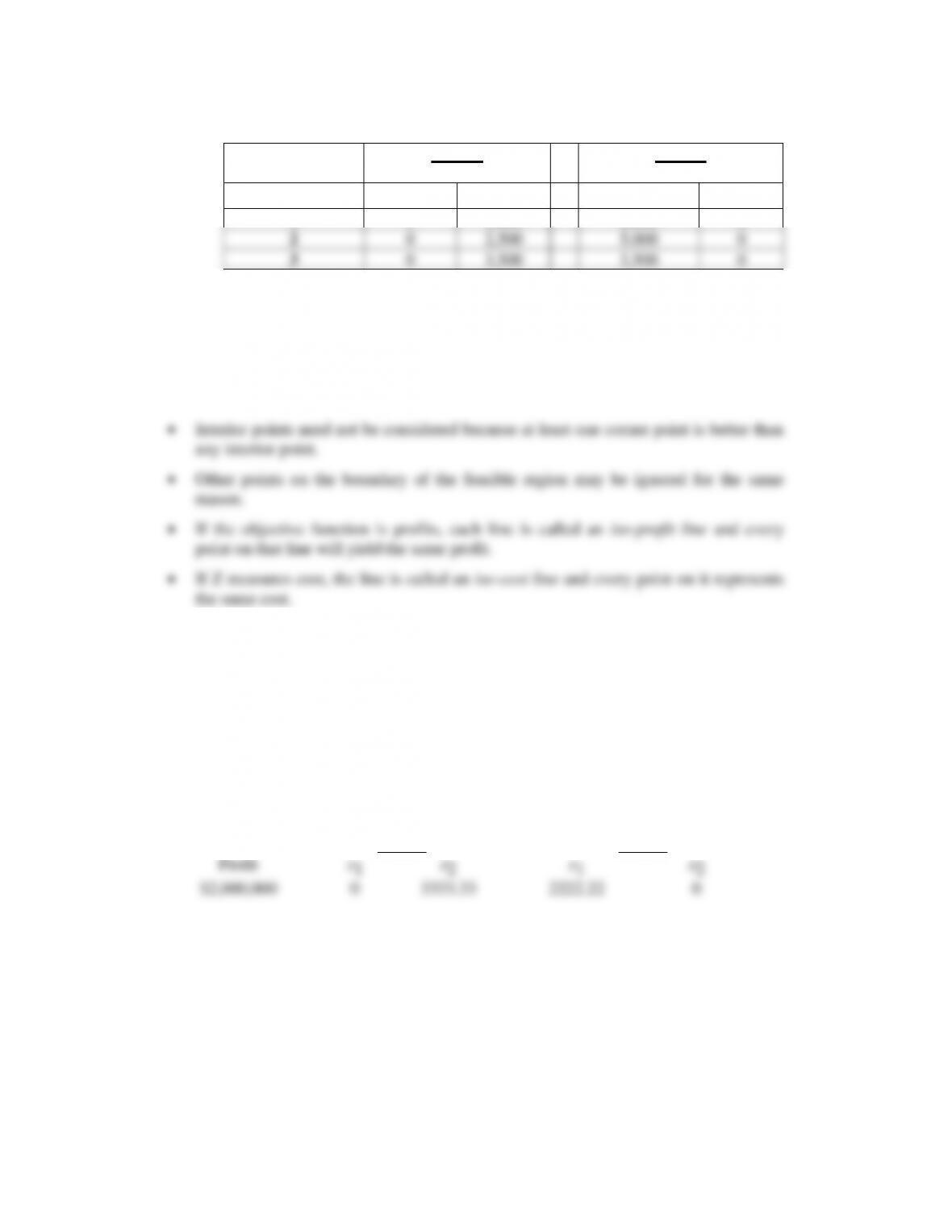
Point 1
Point 2
Profit
x1
x2
x1
x2
$2,000,000
0
3333.33
2222.22
0
e. Find the algebraic solution
• Step 1: Develop an equation with just one unknown. Start by multiplying both sides
by a constant so that the coefficient for one of the two decision variables is identical
in both equations. Then subtract one equation from the other and solve the resulting
equation for its single unknown variable.
• Step 2: Insert this decision variable’s value into either one of the original constraints
and solve for the other decision variable.
• Use Application D.4: Step e for Crandon Manufacturing.
Solve algebraically, with two equations and two unknowns
• Tutor D.2 in MyLab Operations Management provides a new practice example for
finding the optimal solution.
3. Slack and surplus variables
a. A binding constraint is a resource which is completely exhausted when the optimal
solution is used because it limits the ability to improve the objective function.
• Insert the optimal solution into a constraint equation and solve it. If the number on
the left-hand side and the number on the right-hand side are equal, then the constraint
is binding.
• Relaxing a constraint means increasing the right-hand side for a constraint and
decreasing the right-hand side for a constraint. Relaxing a binding constraint means
a better solution is possible. No improvement in the objective function is possible if
the constraint is not binding.
b. Slack is the amount needed to be added to the left-hand side of a constraint to make
both sides equal.
c. Surplus is the amount to subtract from the left hand side of a constraint to make both
sides equal.
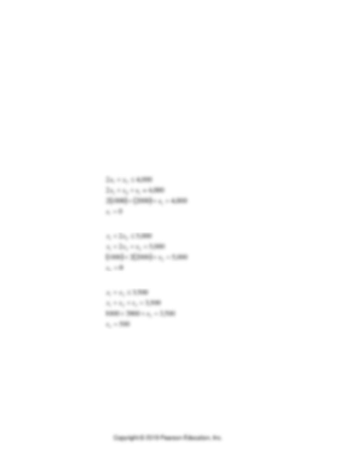
• Use Application D.5: Slack Variables for Crandon Manufacturing.
Find the slack at the optimal solution.
Slack in fabrication at (1000, 2000)
( ) ( )
0
000,4200010002
000,42
000,42
1
1
121
21
=
=++
=++
+
s
s
sxx
xx
Slack in assembly at (1000, 2000)
( ) ( )
0
000,5200021000
000,52
000,52
2
2
221
21
=
=++
=++
+
s
s
sxx
xx
Slack in demand at (1000, 2000)
500
500,320001000
500,3
500,3
3
3
321
21
=
=++
=++
+
s
s
sxx
xx
• Tutor D.3 in MyLab Operations Management provides another practice example for
finding slack.
4. Sensitivity Analysis
a. Rarely are the parameters in the objective function and constraints known with certainty.
b. Usually parameters are just estimates which don’t reflect uncertainties such as
absenteeism or personal transfers.
c. After solving the problem using these estimated values, the analysts can determine how
much the optimal values of the decision variables and the objective function value Z
would be affected if certain parameters had different values. This type of post solution
analysis for answering “what–if” questions is called sensitivity analysis.
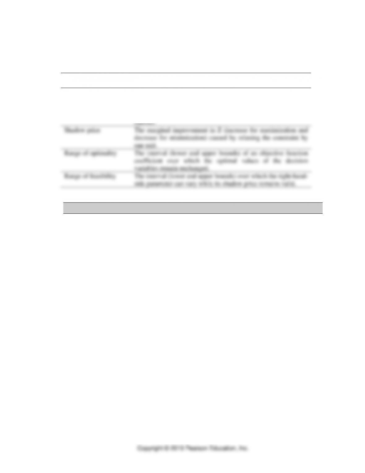
d. Four basic types of sensitivity analysis (table D.1).
Term
Definition
Reduced cost
How much the objective function coefficient of a decision
variable must improve (increase for maximum or decrease for
minimization) before the optimal solution changes and the
decision variable “enters” the solution with some positive
number.
Shadow price
The marginal improvement in Z (increase for maximization and
decrease for minimization) caused by relaxing the constraint by
one unit.
Range of optimality
The interval (lower and upper bounds) of an objective function
coefficient over which the optimal values of the decision
variables remain unchanged.
Range of feasibility
The interval (lower and upper bounds) over which the right-hand-
side parameter can vary while its shadow price remains valid.
4. Computer Analysis
1. Simplex method
a. The simplex method is an iterative algebraic procedure.
b. Graphic analysis gives insight into the logic of the simplex method.
c. The initial feasible solution of the simplex method usually starts out at an initial corner
point. Each subsequent iteration results in an improved intermediate solution which we
have represented graphically by the intersection of two linear constraints. In general, a
corner point has variables greater than 0, where m is the number of constraints.
d. When no further improvement is possible, the optimal solutions have been found and the
algorithm stops.
2. Computer Output
a. Most real-world linear programming problems are solved on a computer, which can
dramatically reduce the amount of time required to solve linear programming problems.
b. POM for Windows in MyLab Operations Management can handle small- to medium-
sized linear programming problems.
c. Microsoft’s Excel Solver offers a second option for similar problem sizes. See the
tutorial in MyLab Operations Management for Supplement E to learn about this second
option.
d. Here we illustrate with POM for Windows.
e. The POM for Windows has two data entry screens
• The Inputs Screen
Asks for the problem’s name
Copyright © 2019 Pearson Education, Inc.
Asks for the number of decision variables and constraints.
Asks whether it is a maximization or minimization problem.
After making these inputs, click the “OK” button to open the next screen which
shows the completed data table.
The user may choose to enter labels for the decision variables, right-hand-
side values, objective function, and constraints.
Slack and surplus variables will be added automatically as needed.
When all of the inputs are made, click the green arrow labeled “Solve”
button in the upper-right corner.
• The Results screen
Click on the Window icon to switch to the Ranging screen (as shown in figure
D.9). The top half deals with the optimal values of the decision variables. Also of
interest are the reduced costs and the lower and upper bounds.
Tips for interpreting the reduced cost information.
(i) The sensitivity number is relevant only for a decision variable that is 0 in
the optimal solution. If the decision variable is greater than 0, ignore the
coefficient sensitivity number.
(ii) It reports how much the objective function coefficient must improve
(increase for maximization problems or decrease for minimization
problems) before optimal solution at some positive level.
Top half also deals with the range of optimality
The bottom half deals with the constraints, including slack or surplus variables
and the original right-hand-side values. Of particular interest are the shadow
prices.
Tips for interpreting its values.
(i) The number is relevant only for binding constraints, where the slack or
surplus variable is 0 in the optimal solution. For a nonbinding constraint,
the shadow price is 0.
(ii) The shadow price as either positive or negative. The sign depends on the
objective function is being maximized or minimized, and whether it is a
constraint or constraint. By ignoring the signs, the value always tells
how much the objective function’s Z value improves (increases for
maximization problems or decreases for minimization problems) by
making the constraint more restrictive by one unit.
• The number of variables in the optimal solution (counting the decision variables,
slack variables, and surplus variables) that are greater than 0 never exceeds the
number of constraints.
• On rare occasions, the number of nonzero variables in the optimal solution can be
less than the number of constraints—a condition called degeneracy. When this
occurs, the sensitivity analysis information is suspect.
f. Stratton Company Example provides the POM for Windows input and output screens.
5. The Transportation Method
1. A special case of linear programming is the transportation problem.
a. Represented as a standard table, sometimes called a tableau.
b. Rows of the table are linear constraints that impose capacity limitations
c. Columns are linear constraints that require a certain demand level to be met.
d. Each cell in the tableau is a decision variable, and a per-unit cost is shown in each cell.
e. The focus in this section is on the setup and interpretation of the problem.
2. Transportation method for Sales and Operations planning
a. Making sure that demand and supply are in balance is central to sales and operations
planning (SOP), and the transportation method can be applied to it.
b. Helpful in determining anticipation inventories.
c. Transportation method for production planning is based on the several assumptions
• Demand forecast is available for each period, along with a possible workforce
adjustment plan.
• Capacity limits on overtime and the use of subcontractors also are needed for each
period.
• All costs are linearly related to the amount of goods produced
d. Example D.6 Tru-Rainbow Company demonstrates this approach using the
Transportation Method (Production Planning) module in the POM for Windows package.
e. Application D.6: The Transportation Method of Production Planning
The Bull Grin Company makes an animal-feed supplement. Sales are seasonal, but Bull
Grin’s customers refuse to stockpile the supplement during slack sales periods; they insist
on shipments according to their schedules to stockpile the supplement during slack sales
periods and won’t accept backorders. The reactive alternatives that they use, in addition
to work-force variation, are regular time, overtime, subcontracting, and anticipation
inventory. Backorders are not allowed.
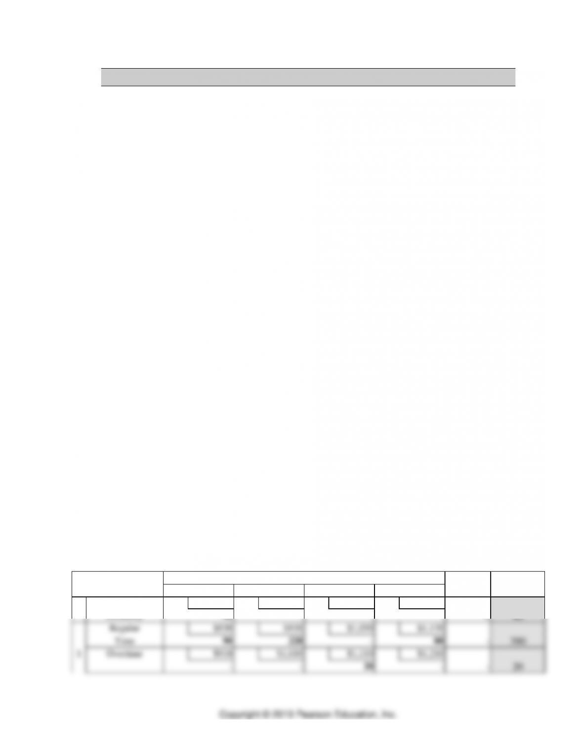
Complete the tableau given below by entering the cost per pound produced with each
production alternative to meet demand in each period. Bull Grin employs workers who
produce 1,000 pounds of supplement for $830 on regular time and $910 on over-time.
Holding 1000 pounds of feed supplement in inventory per quarter costs $100. There is no
cost for unused regular-time, overtime or subcontracting capacity. (The entire solution is
shown; students complete highlighted sections)
Quarter
Unused
Total
Alternatives
1
2
3
4
Capacity
Capacity
Beginning
$0
$100
$200
$300
Inventory
40
0
40
Regular
$830
$930
$1,030
$1,130
Time
90
220
–
80
–
390
1
Overtime
$910
$1,010
$1,110
$1,210
–
–
20
–
–
20
Subcontract
$1,000
$1,100
$1,200
$1,300
–
–
–
–
30
30
Regular
$99,999
$830
$930
$1,030
Time
180
220
–
400
2
Overtime
$99,999
$910
$1,010
$1,110
20
–
20
Subcontract
$99,999
$1,000
$1,100
$1,200
30
–
30
Regular
$99,999
$99,999
$830
$930
Time
460
–
460
3
Overtime
$99,999
$99,999
$910
$1,010
20
–
20
Subcontract
$99,999
$99,999
$1,000
$1,100
30
–
30
Regular
$99,999
$99,999
$99,999
$830
Time
380
–
380
4
Overtime
$99,999
$99,999
$99,999
$910
20
–
20
Subcontract
$99,999
$99,999
$99,999
$1,000
30
–
30
Demand
130
400
800
510
30
1,870
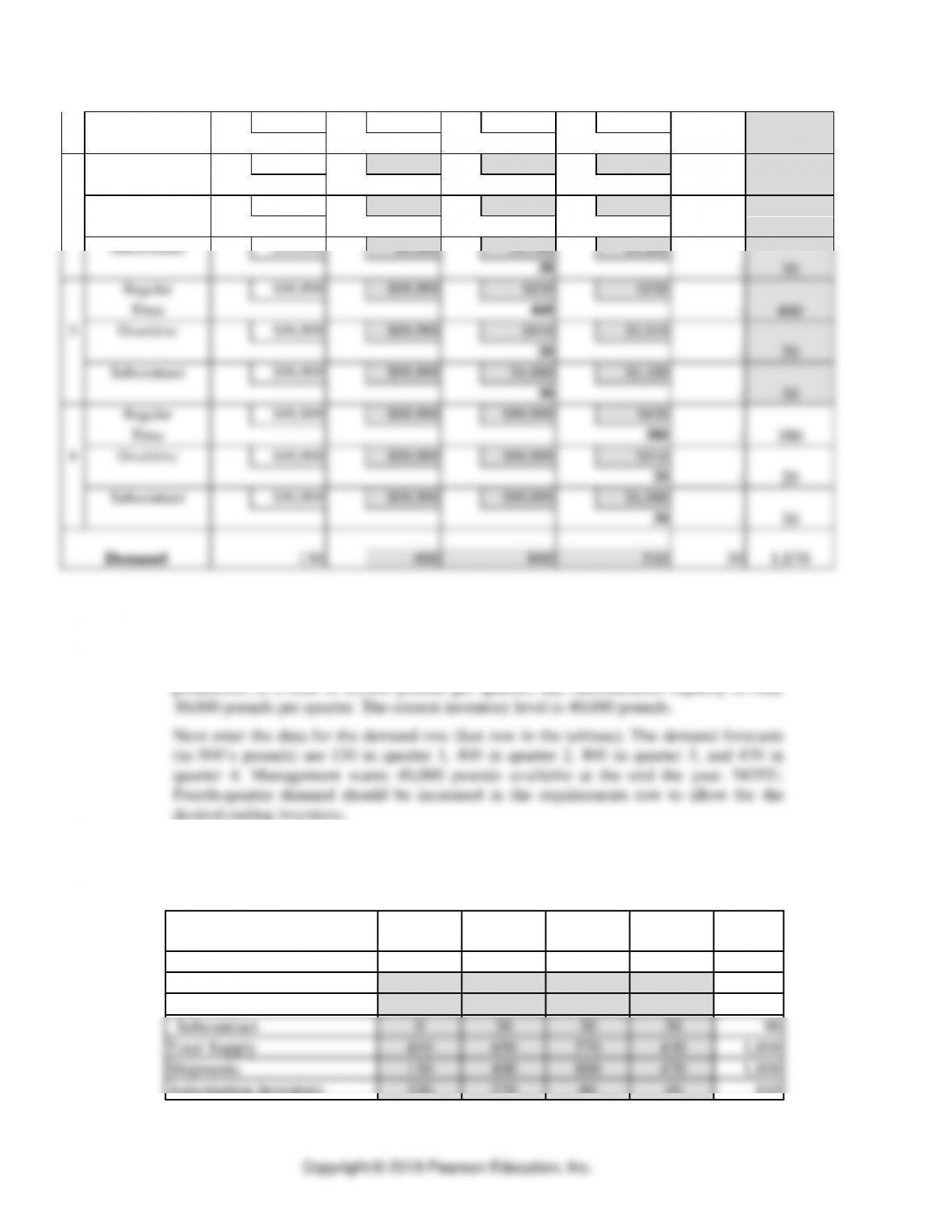
Now enter data for the capacity column of the tableau (final column to right). For
simplicity, enter the data as thousands of pounds. The work-force plan being
investigating now would provide regular-time capacities (in 000’s pounds) of 390 in
quarter 1, 400 in quarter 2, 460 in quarter 3, and 380 in quarter 4. Overtime is limited to
What production levels, shipments, and anticipation inventories are called for by the
optimal solution shown as bold numbers in the tableau above?
Quarter 1
Quarter 2
Quarter 3
Quarter 4
Totals
Production
Regular-time
390
400
460
380
1,630
Overtime
20
20
20
20
80
Subcontract
0
30
30
30
90
Total Supply
410
450
570
430
1,800
Shipments
130
400
800
470
1,800
Anticipation Inventory
320
370
80
40
810
(Students complete the highlighted sections.)
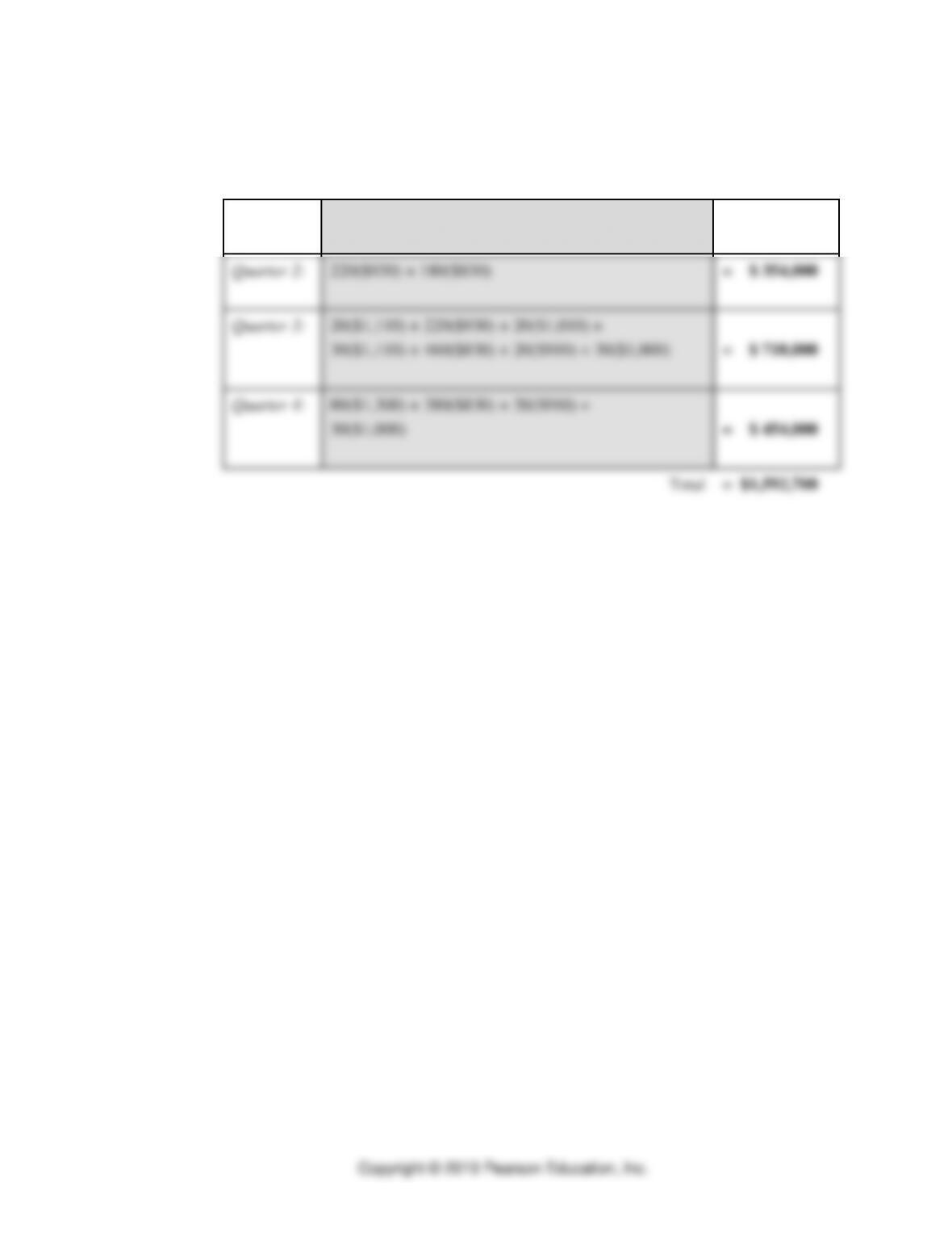
What is the total cost of the optimal solution, except for the cost of hiring and layoffs?
Quarter 1:
40($0) + 90($830)
= $ 74,700
Quarter 2:
220($930) + 180($830)
= $ 354,000
Quarter 3:
20($1,110) + 220($930) + 20($1,010) +
30($1,110) + 460($830) + 20($910) + 30($1,000)
= $ 710,000
Quarter 4:
80($1,300) + 380($830) + 20($910) +
30($1,000)
= $ 454,000
Total
= $1,592,700