
Chapter
8 Forecasting
Forecasting
1. What is a forecast?
2. Forecasts are critical inputs to business plans, annual plans, and budgets.
a. Finance:
b. Human resources:
c. Marketing:
d. Operations and supply chain managers:
3. Managers throughout the organization make forecasts on many different variables other than
future demand, such as:
1. Managing Demand
1. There are five basic patterns of most demand time series.
a.
b.
c.
d.
e.
2. Demand management: the process of changing demand patterns using one or more demand
options – list 8 demand options:
a.
b.
c.
d.
e.
f.
g.
h.

2. Key Decisions on Making Forecasts
1. Deciding what to forecast
2. Choosing the type of forecasting technique
a. Judgment methods
b. Causal methods
c. Time-series analysis
d. Trend projection using regression
3. Forecast Error
1. Definition and formula for forecast error
2. Types of forecast errors
a. Bias
b. Random
3. Cumulative sum of forecast error
a. Cumulative forecast error (bias):
=
=
n
tt
ECFE
1
b. Average forecast error (mean bias):
n
CFE
E=
4. Dispersion of Forecast Errors
a. Mean squared error:
n
E
MSE
n
tt
=
=1
2
b. Standard deviation:
( )
1
1
2
−
−
=
=
n
EE
n
tt

c. Mean absolute deviation:
n
E
MAD
n
tt
=
=1
5. Mean Absolute Percent Error:
a. Mean absolute percent error:
( )
n
DE
MAPE
n
ttt
=
=1
100/
6. Example 8.1: Calculating Forecast Error Measures
A forecasting procedure has been used for the last 8 months, with the following results.
Evaluate how well the procedure is doing, by finishing the following table and then
computing the different forecast error measures.
Month
Demand
(Dt)
Forecast
(Ft)
Error
(Et)
Error
Squared
(Et2)
Absolute Error
(Et
)
Absolute Percent
Error
(Et
/ Dt)100
1
200
225
–25
____
____
____%
2
240
220
20
____
____
____
3
300
285
15
____
____
____
4
270
290
–20
____
____
____
5
230
250
−20
400
20
8.7
6
260
240
20
400
20
7.7
7
210
250
−40
1600
40
19.0
8
275
240
35
1225
35
12.7
Totals
=CFE
=E
=MSE
=
=MAD
=MAPE
4. Judgment Methods
Types of judgment methods
1.
2.
3.
4.
5. Causal Methods: Linear Regression
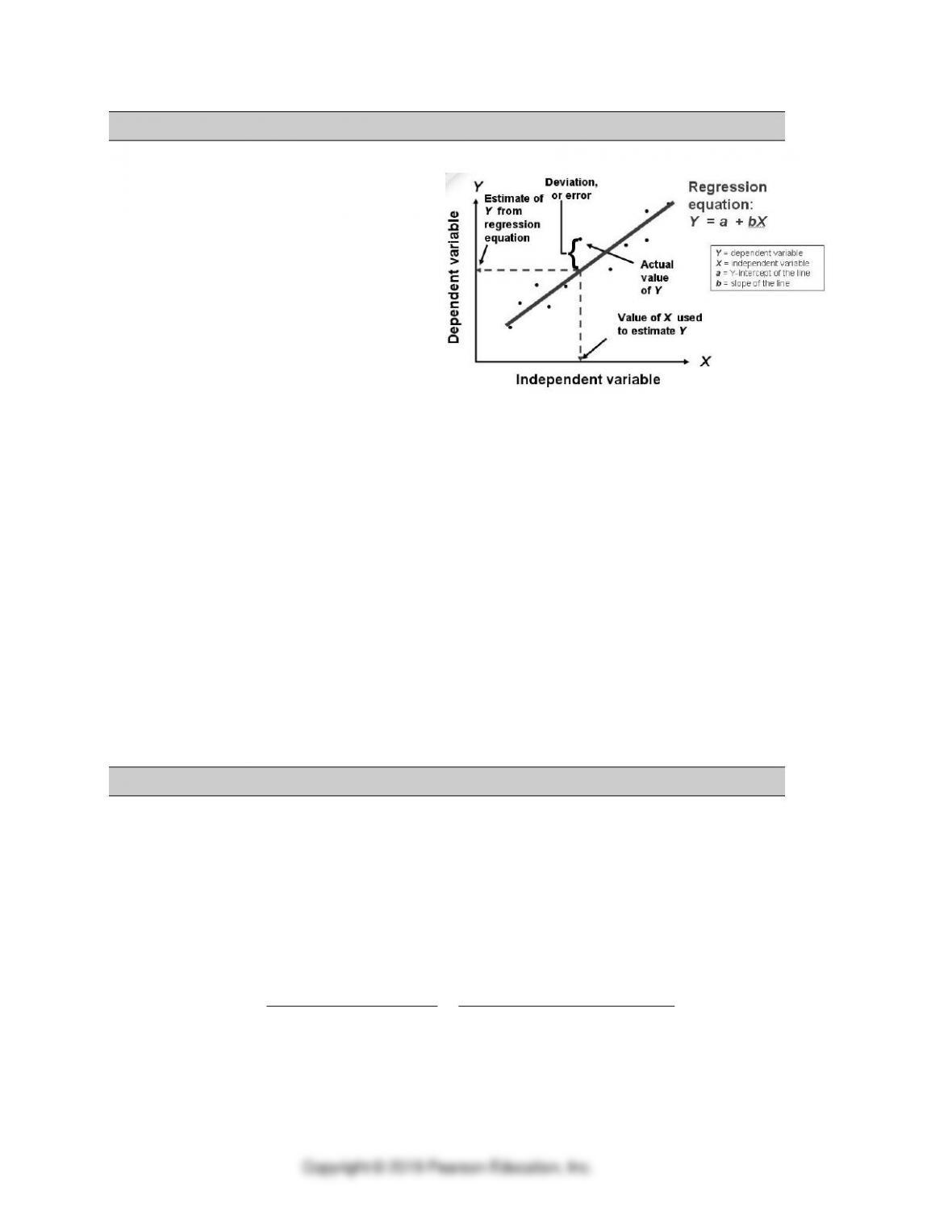
1. Linear regression
a. Definition
b. Dependent variable and independent
variables
c. In models with only one independent
variable, the theoretical relationship is
a straight line:
Y= a + bX
where
Y =
dependent variable
X =
independent variable
a =
Y-intercept of the line
b =
slope of the line
2. Sample correlation coefficient, r
3. Sample coefficient of determination, r2
4. Standard error of the estimate, syx
5. Forecasting with linear regression
6. Example 8.2: Using Linear Regression to Forecast Product Demand
6. Time-Series Methods
1. Naive forecast. Forecast = Dt
2. Horizontal patterns: Estimating the average
a. Simple moving average
1. Forecasting formula:
n
DDDD
n
demands n last of Sum
Fntttt
t121
1+−−−
+
++++
==
where
Dt =
actual demand in period t
n =
total number of periods in the average
Ft+1 =
forecast for period t+1

2. Example 8.3: Using the Moving Average Method to Estimate Average Demand
3. Application 8.1: Estimating with Simple Moving Average
We will use the following customer-arrival data in this application.
Month
Customer arrivals
1
800
2
740
3
810
4
790
Use a three-month moving average to forecast customer arrivals for month 5.
=
++
=3
234
5
DDD
F
Forecast for month 5 is _____ customer arrivals.
If the actual number of arrivals in month 5 is 805, what is the forecast for month 6?
=
++
=3
345
6
DDD
F
Forecast for month 6 is _____ customer arrivals.
Given the three-month moving average forecast for month 5, and the number of
patients that actually arrived (805), what is the forecast error?
=
5
E
b. Weighted moving averages. Ft+1 = W1Dt + W2Dt–1 +…+WnDt –n+1
1. Application 8.2: Estimating with Weighted Moving Average
Revisiting the customer arrival data in Application 8.1. Let W1 = 0.50, W2 = 0.30,
and W3 = 0.20. Use the weighted moving average method to forecast arrivals for
month 5.
( ) ( ) ( )
=++=++= ___20.0___30.0___50.0
2332415 DWDWDWF
Forecast for month 5 is _____ customer arrivals.
If the actual number of arrivals in month 5 is 805, what is the forecast error?
=
5
E
What is the forecast for month 6?
( ) ( ) ( )
=++=++= ___20.0___30.0___50.0
3342516 DWDWDWF
Forecast for month 6 is _____ customer arrivals.
c. Exponential smoothing
1. Formula:
( ) ( )( )
tt
t
FD
period last calculated Forecastperiod this DemandF
)1(
1
1
−+=
−+=
+
2. An equivalent formula is:
( )
tttt FDFF −+=
+
1
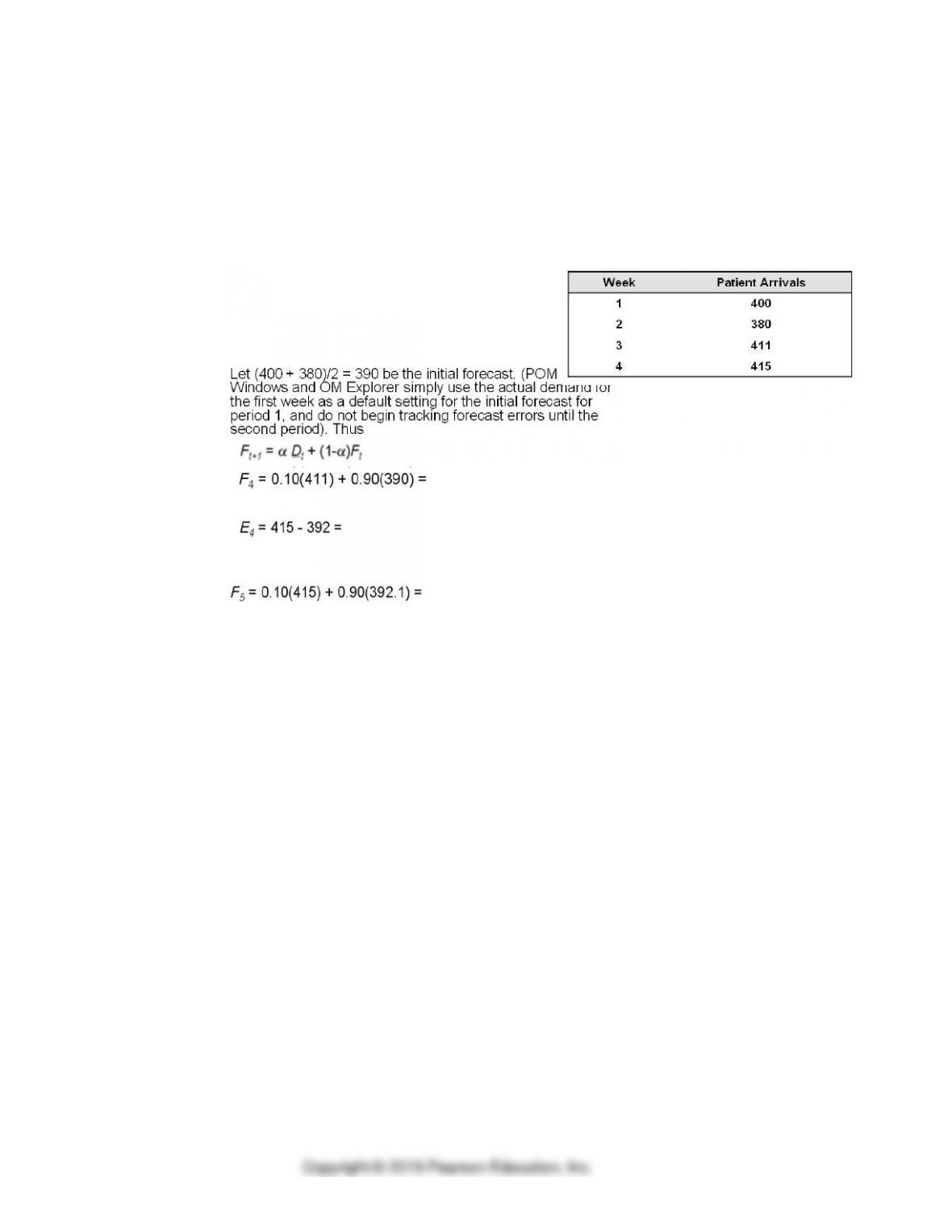
3. Example 8.4: Using Exponential Smoothing to Estimate Average Demand
• Reconsider the patient arrival data in Example
8.3. It is now the end of week 3. Using =
0.10, calculate the exponential smoothing
forecast for week 4.
• What is the forecast error for week 4 if the actual demand turned out to be 415?
• What is the forecast for week 5?
A
a. Application 8.3 Estimating with Exponential Smoothing
Suppose that there were 790 customer arrivals in month 4 (D4), whereas the forecast
was for 783 arrivals. Use exponential smoothing with α=0.20 to compute the forecast
for month 5.
( )
=−+=
+tttt FDFF
1
Forecast for month 5 is ___ customer arrivals.
If the actual number of arrivals is 805, what is the forecast error?
=
5
E
What is the forecast for month 6?
( )
=−+=
+tttt FDFF
1
Forecast for month 6 is ___ customer arrivals.
3. Trend Patterns: Using Regression
a. Define and state form of regression equation
b. Example 8.5: Using Trend Projection with Regression to Forecast a Demand Series
with a Trend
Graphs and Detailed Analysis:
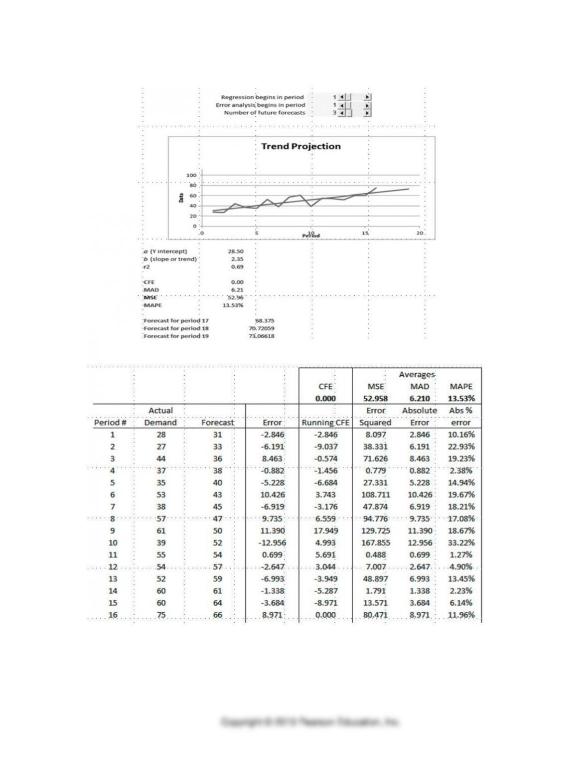
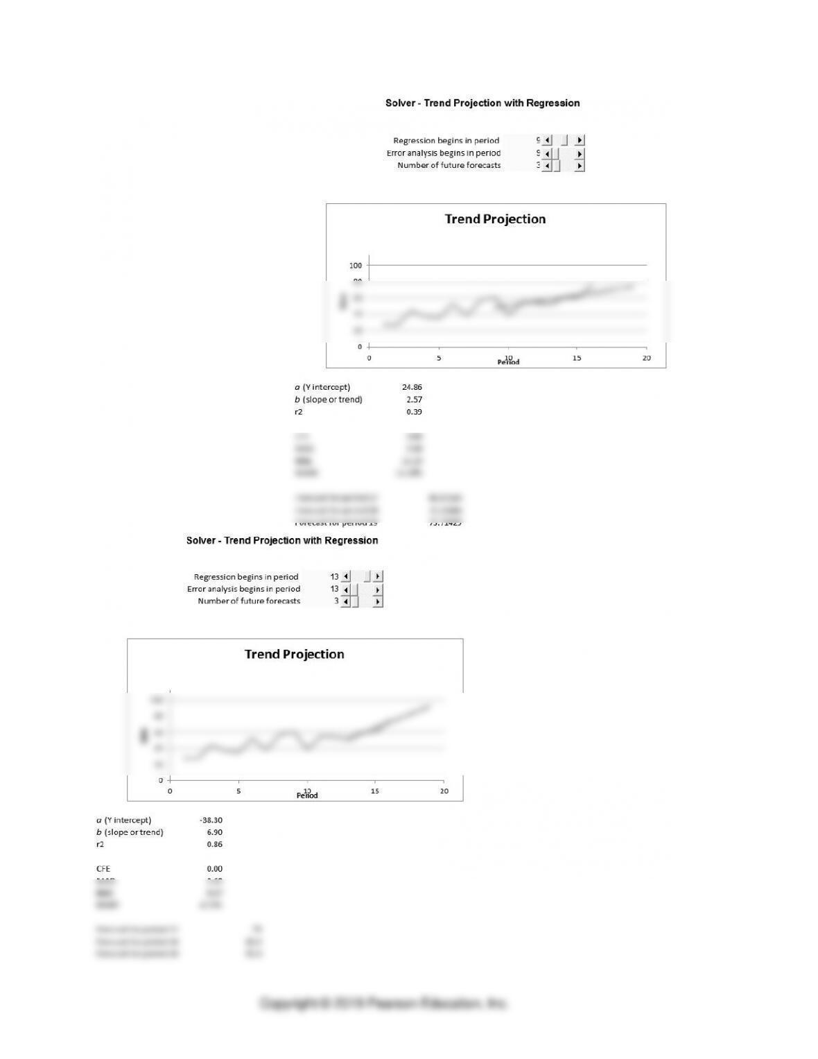
c. Consider other models by varying the number of periods in the regression, making the
model more or less adaptive.
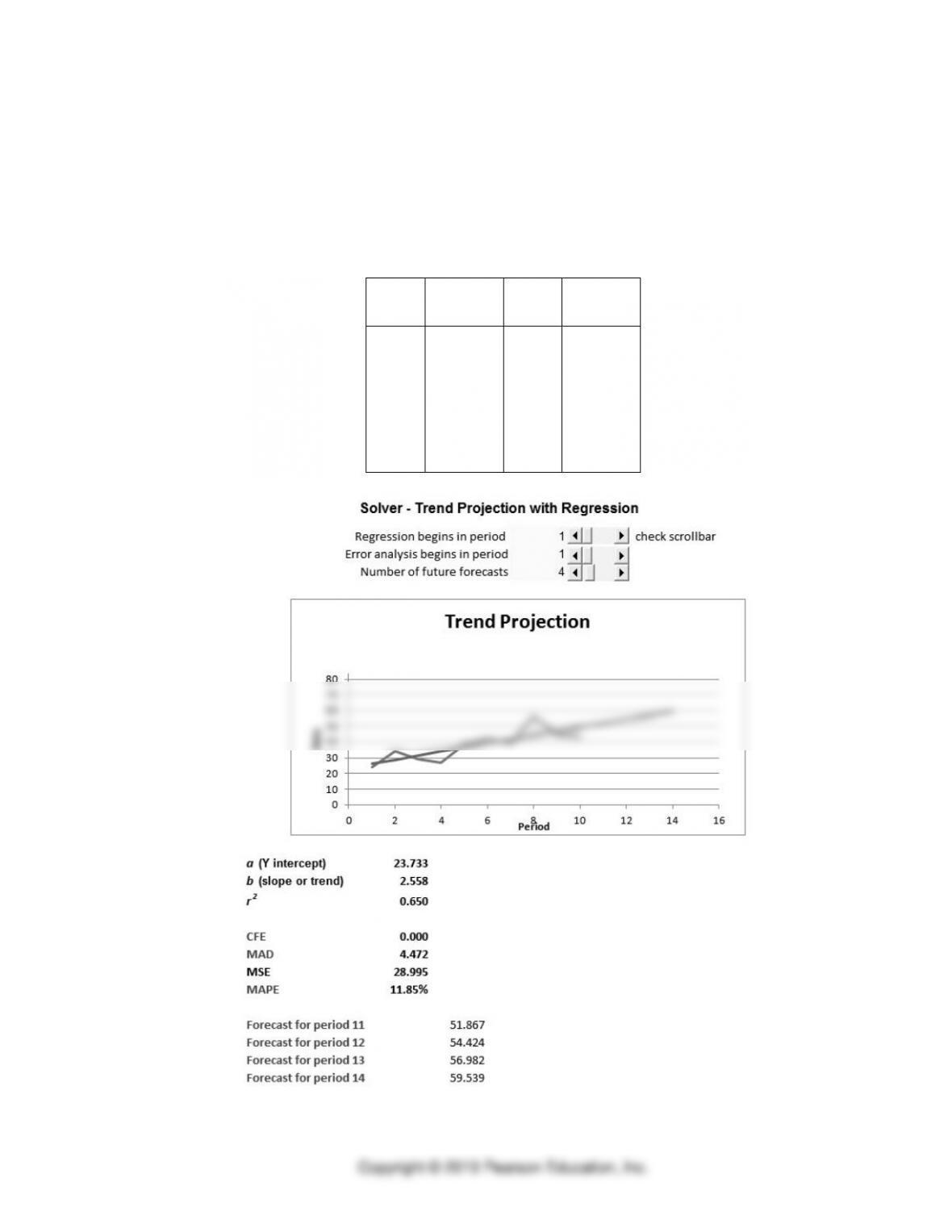
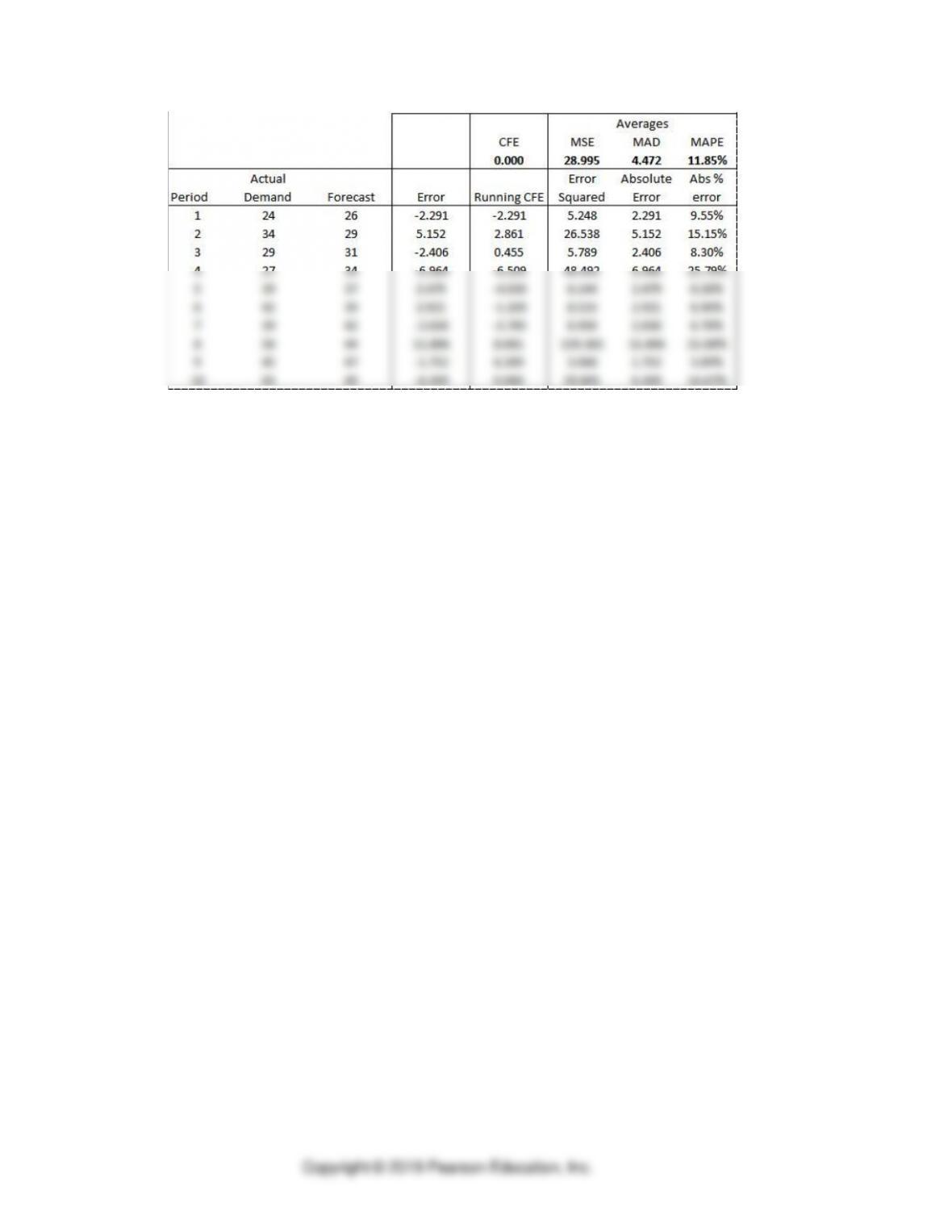
d. Application 8.4: Using Trend Projection with Regression to Forecast a Demand
Series with a Trend
Use OM Explorer to project the following weekly demand data using trend projection
with regression. What is the forecasted demand for periods 11-14?
Week
Demand
Week
Demand
1
2
3
4
5
24
34
29
27
39
6
7
8
9
10
42
39
56
45
43
4. Seasonal patterns: Using Seasonal Factors
a. Multiplicative and Additive Seasonal Methods
b. Multiplicative seasonal method calculates seasonal factors that are then multiplied by an
estimate of the average demand to arrive at a seasonal forecast.
a) Step 1:
b) Step 2:
c) Step 3:
d) Step 4:
c. Example 8.6 Using the Multiplicative Seasonal Method to Forecast the Number of
Customers.
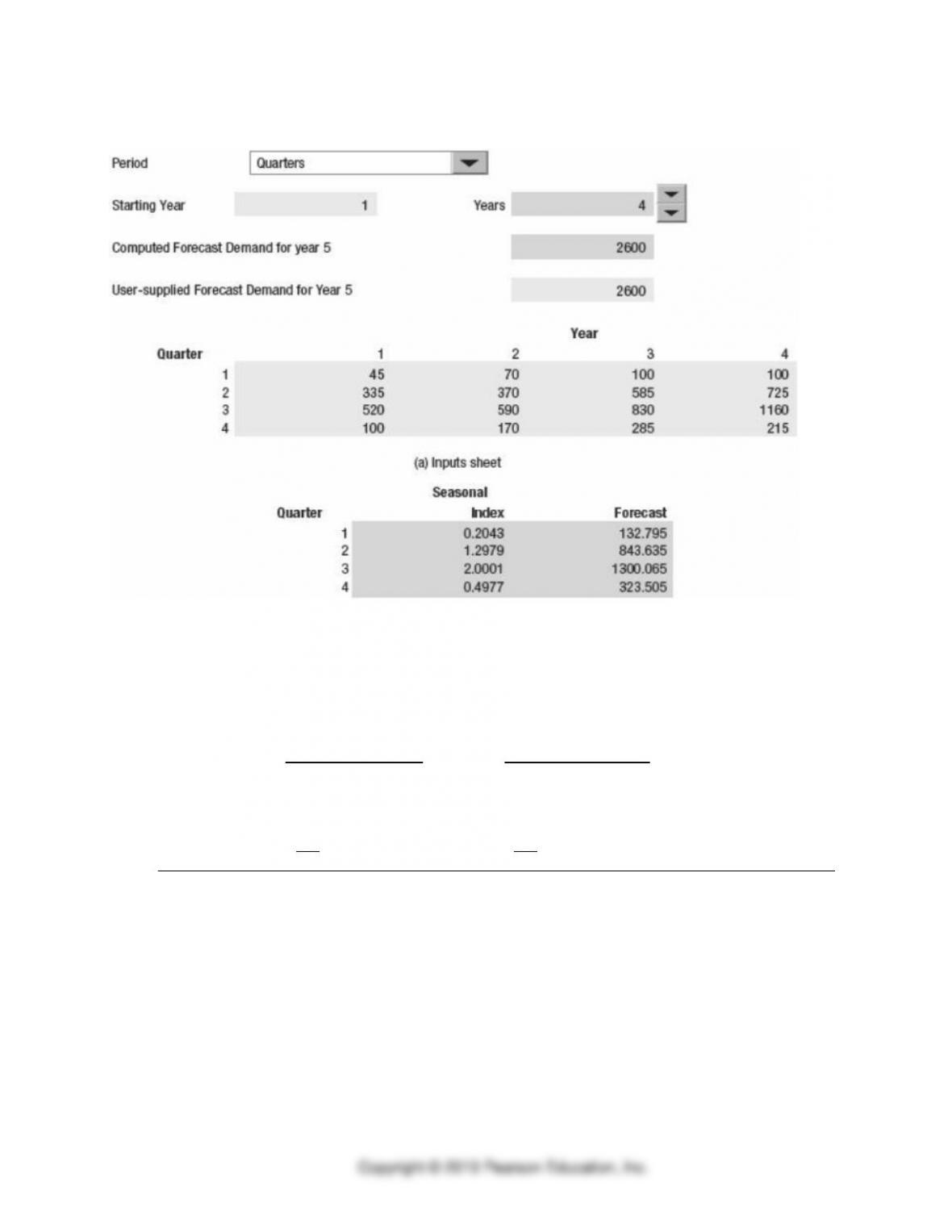
d. Application 8.5: Forecasting Using the Multiplicative Seasonal Method with manual
calculations
Suppose the multiplicative seasonal method is being used to forecast customer demand. The
actual demand and seasonal indices are shown below.
Year 1 _
Year 2 _
Average
Quarter
Demand
Index
Demand
Index
Index
1
100
0.40
192
0.64
0.52
2
400
1.60
408
1.36
1.48
3
300
1.20
384
1.28
1.24
4
200
0.80
216
0.72
0.76
Avg.
250
300
If the projected demand for Year 3 is 1,320 units (or 330 units per quarter), what is the
forecast for each quarter of that year?
Forecast for Quarter 1 =
Forecast for Quarter 2 =
Forecast for Quarter 3 =
Forecast for Quarter 4 =
e. Multiplicative versus additive methods
5. Criteria for Selecting Time-Series Methods

a. Forecast error measures include
o
o
o
o
o
b. Using Statistical criteria:
o For more stable demand patterns, use…
o For more dynamic demand patterns, use …
c. Using a Holdout Sample
d. Using a Tracking Signal
7. Insights into Effective Demand Forecasting
1. Big Data
a) Three Vs:
•
•
•
2. A typical forecasting process
a) Step 1:
b) Step 2:
c) Step 3:
d) Step 4:
e) Step 5:
f) Step 6:

3. Using Multiple Forecasting Methods
a) Combination forecasts
b) Focus forecasting
4. Adding collaboration to the Process:
a) Collaborative planning, forecasting, and replenishment (CPFR)
• Strategy and planning
• Demand and supply management
• Execution
• Analysis
5. Forecasting as a nested process