Unlock document.
This document is partially blurred.
Unlock all pages and 1 million more documents.
Get Access
Forecasting ⚫ CHAPTER 8 ⚫
8-41
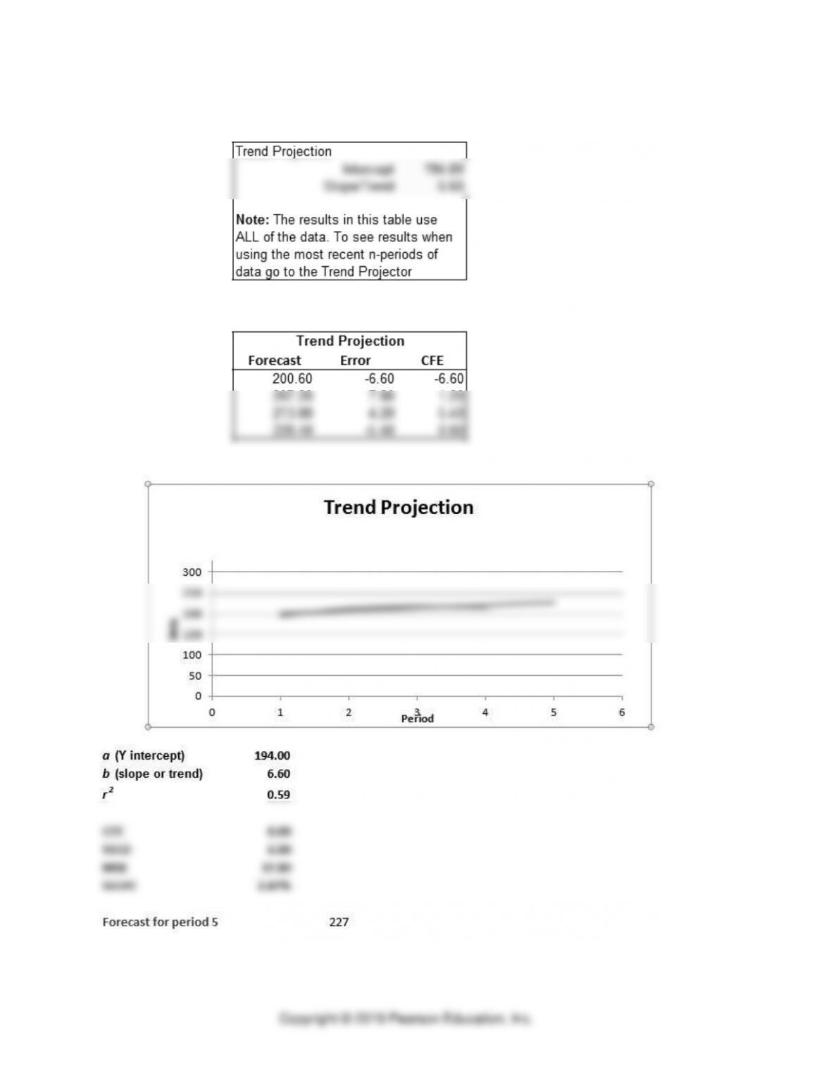
One way to estimate the total demand for cycle 5 is to use OM Explorer’s Trend Projection
routine in the Time Series Solver. Here we get the following results:
PART 2 Managing Customer Demand
8-42
Thus the average demand per period for the 5th cycle is forecast to be 227 / 5 = 45.4. Applying the
seasonal indexes, we get:
Actual
Seasonal
Forecast
Period
Cycle 5
Index
Cycle 5
21
42
0.9186
42
22
45
0.9155
42
23
41
0.8712
39
24
38
0.9746
44
25
??
1.3202
60
227
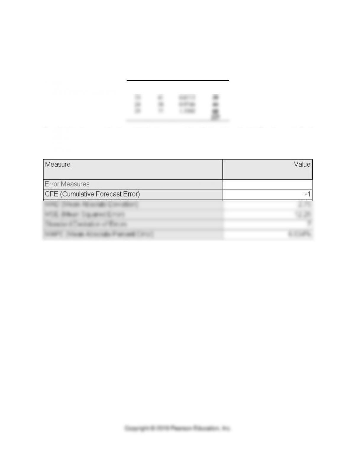
To calculate the errors for the multiplicative seasonal method, at least for the first four periods of
the 5th cycle, we use the Error Analysis module of POM for Windows, with the following results:
At least over this limited sample, the multiplicative seasonal method performs better than the
Combination method because it accounts for the peak in the last period of each cycle.
Forecasting ⚫ CHAPTER 8 ⚫
8-43
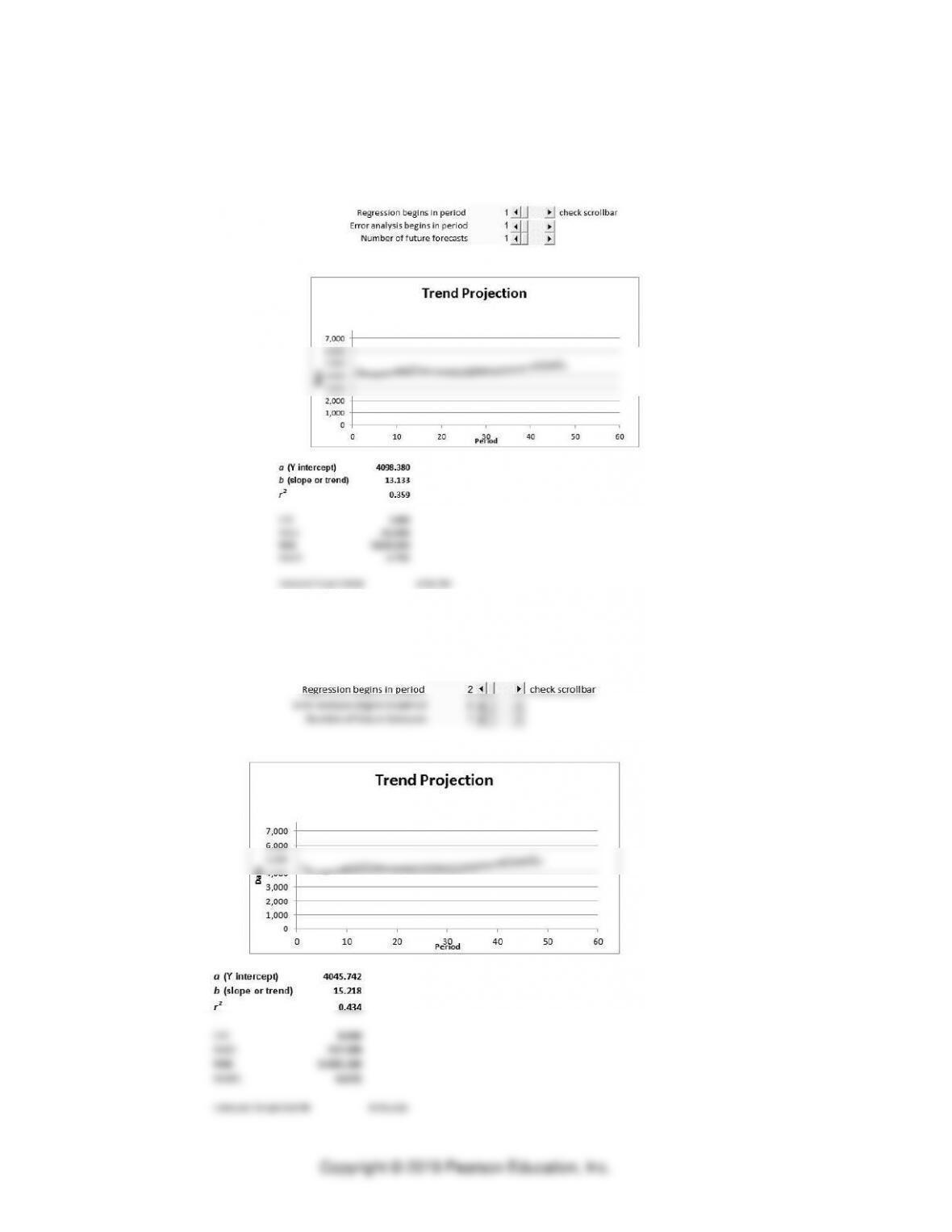
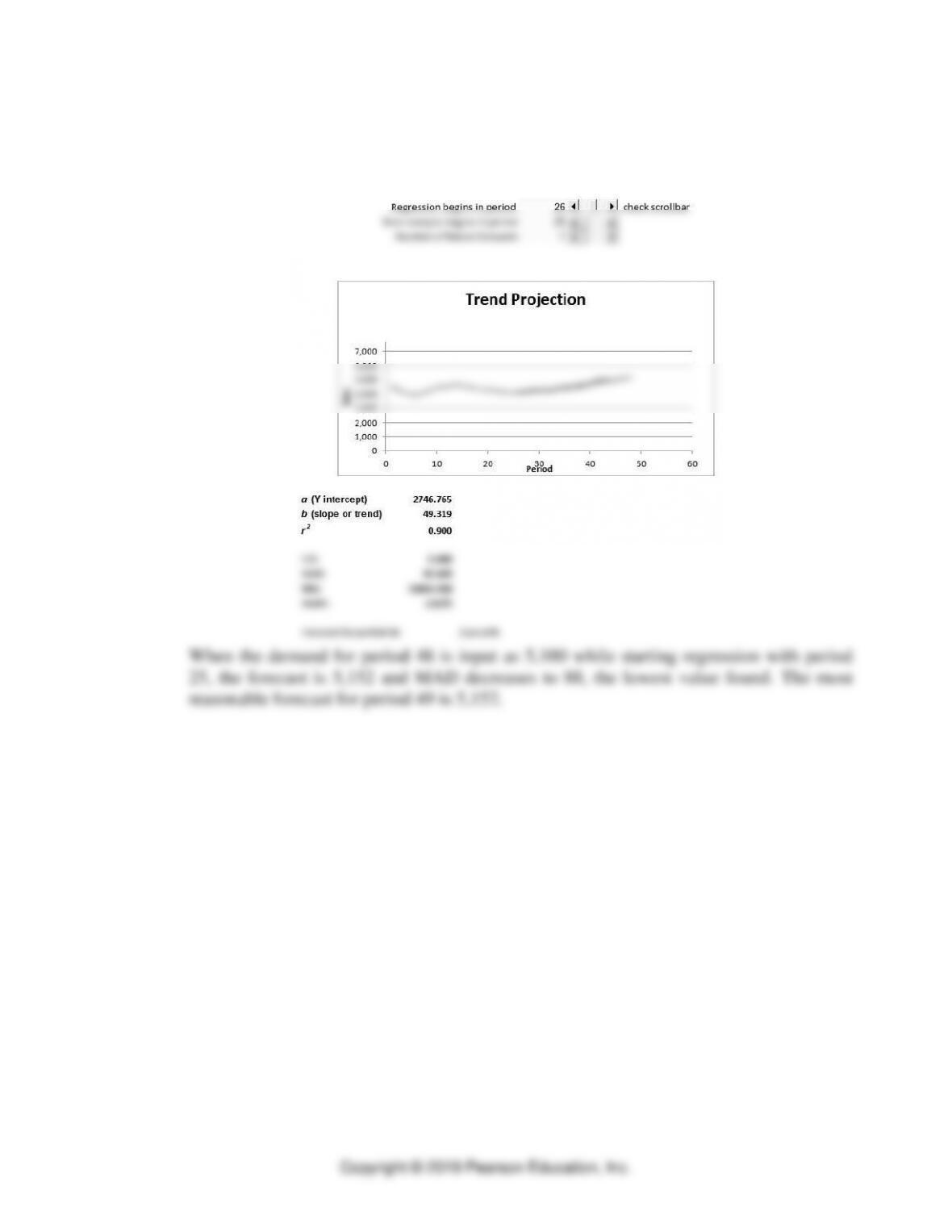
26. Air visibility
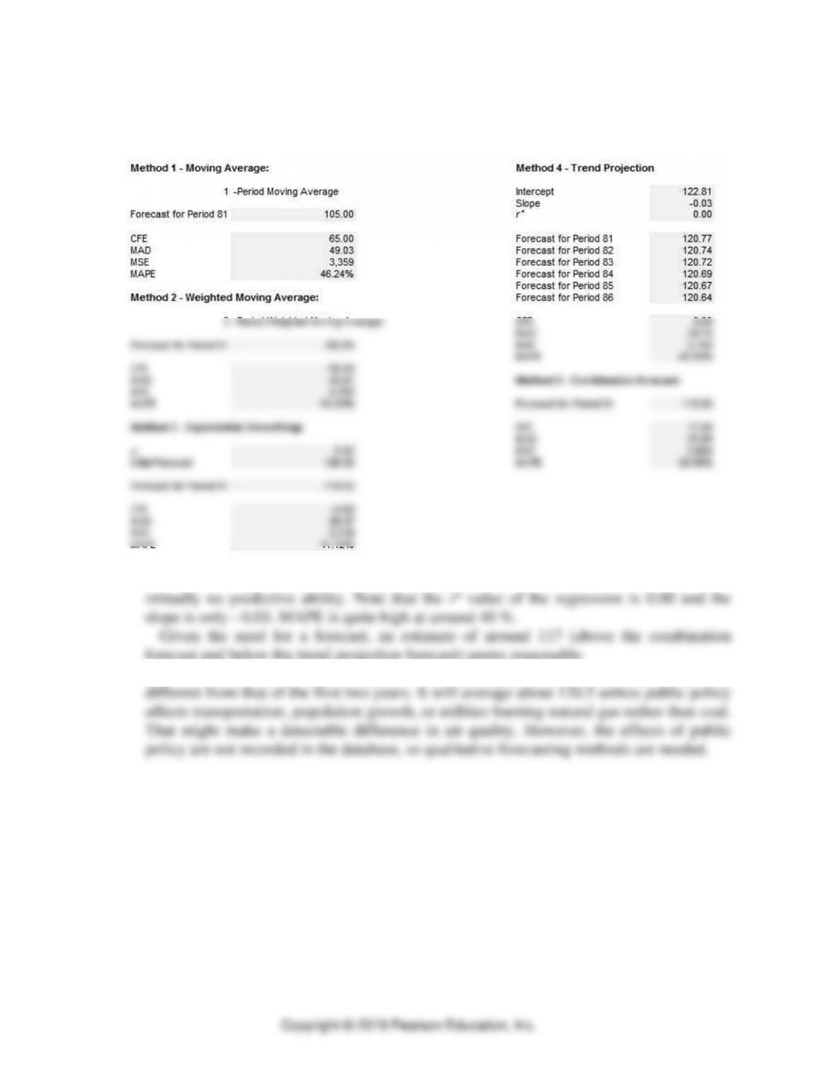
a. Below is the analysis using the Time Series Forecasting Solver of OM Explorer.
The Trend Projection and Combination models give the best results, but they offer
forecast and below the trend projection forecast) seems reasonable.
b. There is no reason to support expectations for air quality in the third year to be any
PART 2 Managing Customer Demand
8-44
27. Flatlands Public Power District
The historical data show both trend and seasonal components. We will use the multiplicative
seasonal method to forecast demand for the next year, then look for a low-demand period of
two weeks during which the Comstock plant can be serviced. Weeks 7 and 8 look like the best
two-week period to schedule maintenance.
Demand
Seasonal
Demand
Seasonal
Demand
Seasonal
Demand
Seasonal
Demand
Seasonal
Week
Year 1
Index
Year 2
Index
Year 3
Index
Year 4
Index
Year 5
Index
1
2,050
0.1017
2,000
0.0959
1,950
0.0922
2,100
0.1010
2,275
0.1064
2
1,925
0.0955
2,075
0.0995
1,800
0.0851
2,400
0.1154
2,300
0.1076
3
1,825
0.0906
2,225
0.1067
2,150
0.1017
1,975
0.0950
2,150
0.1006
4
1,525
0.0757
1,800
0.0863
1,725
0.0816
1,675
0.0805
1,525
0.0713
5
1,050
0.0521
1,175
0.0564
1,575
0.0745
1,350
0.0649
1,350
0.0632
6
1,300
0.0645
1,050
0.0504
1,275
0.0603
1,525
0.0733
1,475
0.0690
7
1,200
0.0596
1,250
0.0600
1,325
0.0626
1,500
0.0721
1,475
0.0690
8
1,175
0.0583
1,025
0.0492
1,100
0.0520
1,150
0.0553
1,175
0.0550
9
1,350
0.0670
1,300
0.0624
1,500
0.0709
1,350
0.0649
1,375
0.0643
10
1,525
0.0757
1,425
0.0683
1,550
0.0733
1,225
0.0589
1,400
0.0655
11
1,725
0.0856
1,625
0.0779
1,375
0.0650
1,225
0.0589
1,425
0.0667
12
1,575
0.0782
1,950
0.0935
1,825
0.0863
1,475
0.0709
1,550
0.0725
13
1,925
0.0955
1,950
0.0935
2,000
0.0946
1,850
0.0889
1,900
0.0889
Total
20,150
20,850
21,150
20,800
21,375
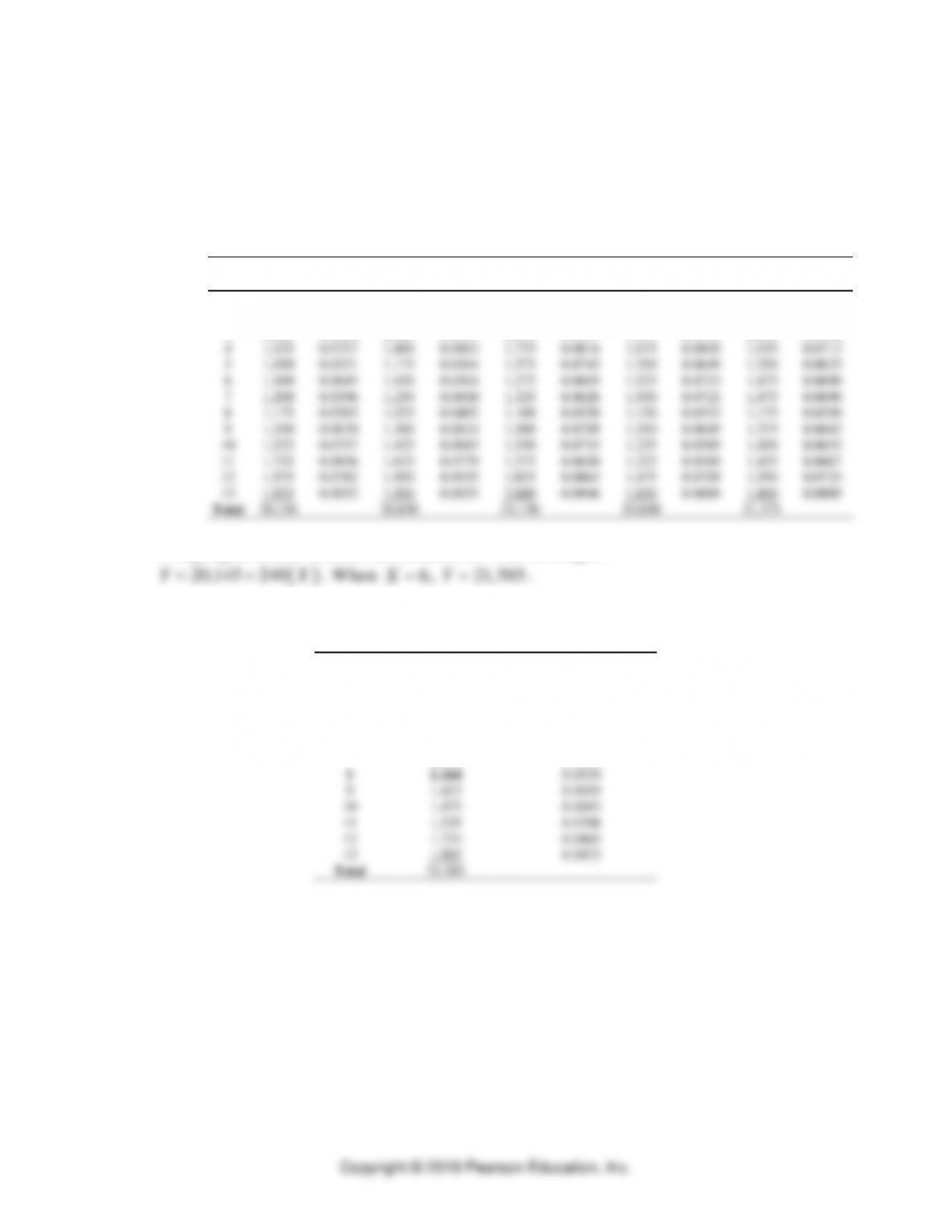
Using regression to forecast the demand for Year 6, we get :
( )
20,145 240YX=+
. When
X=6
,
21,585Y=
.
Using this annual demand forecast, we calculate the weekly breakdown as :
Week
Demand Year 6
Average Seasonal Index
1
2,147
0.0995
2
2,172
0.1006
3
2,135
0.0989
4
1,707
0.0791
5
1,343
0.0622
6
1,371
0.0635
7
1,396
0.0647
8
1,164
0.0539
9
1,422
0.0659
10
1,475
0.0683
11
1,529
0.0708
12
1,733
0.0803
13
1,992
0.0923
Total
21,585
Forecasting ⚫ CHAPTER 8 ⚫
8-45
28. Manufacturing firm
Using the Trend Projection with Regression Solver, we get the following results.
a. The following output makes a forecast of 4,729 units for December of Year 4.
b. The forecast is 4,791 for period 49, up by 63 units. This is quite a jump, and the error
measures have also decreased. For example, MAD drops from 210 to 207. These results
are somewhat surprising, although the actual demand was quite a bit higher than
forecast. Regression can be quite adaptive.
PART 2 Managing Customer Demand
8-46
c. Starting again, but with regression beginning with period 25, the forecast for December
of Year 4 is 5,114 units, as opposed to the 4,729 units forecast when the regression
began with period 1. Error terms are also lower, with MAD down from 210 to 91.

Forecasting ⚫ CHAPTER 8 ⚫
8-47
CASE: YANKEE FORK AND HOE COMPANY
A. Synopsis
Yankee Fork and Hoe is a company that produces garden tools for a mature, price-sensitive
market in which customers also want on-time delivery. Recently customers have been
complaining about late shipments. The president has hired a consultant to look into the
problem. The consultant traces the production planning process and its reliance on accurate
forecasts. The consultant must make a recommendation to management.
B. Purpose
This case provides the basis for a discussion of the need for accurate forecasts in an industry
where low-cost production is critical. It also contains sufficient data to enable the student to
generate forecasts for each month of the following year. Specifically, the case can be used
to:
1. Discuss the effects of poor forecasts on capacities and schedules.
2. Discuss the choice of the proper data to use for forecasts.
3. Quantitatively analyze forecasting data and provide forecasts for the following year.
C. Analysis
Yankee Fork and Hoe is experiencing two major problems with the current forecasting
system. First, the production department is unaware of how marketing arrives at its
forecasts. Production views the forecasts as the result of an overinflated estimate of actual
customer demand. However, the forecasting technique in use by the marketing department is
based on actual shipments rather than on actual demand. Second, marketing, in its desire to

PART 2 Managing Customer Demand
8-48
reflect production capacity, is compounding the problems experienced by Yankee Fork and
Hoe by trying to rectify past problems. Although marketing adjusts for shortages in the
actual shipment data, it is still reflecting past problems and not future demand. If Yankee
would move to a system that utilizes past demand to forecast future demand, production
would be able to schedule bow rake production more effectively. In addition, production
must be aware of how the forecasts are made and what information is being provided so that
arbitrary adjustments are no longer needed.
A forecasting system based on actual demands requires careful analysis of Exhibit TN. 1. It is
apparent that the bow rake experiences seasonal demand. It is also obvious that there is an
upward trend in the annual demand. A forecasting system that recognizes both of these factors
is desirable. To arrive at the average monthly demand for year 5, the average increase in the
average monthly demands was determined to be 2,589 units. Therefore the average monthly
demand for year five is 45,928 + 2,589 = 48,517. This value is then multiplied by the average
seasonal factors (see Exhibit TN.2) to arrive at the forecast shown in Exhibit TN.1. Exhibits
TN.3 and TN.4 show graphs of the series.
D. Recommendations
The recommendations to management could include the following:
1. Improve the lines of communication between marketing and production regarding the
preparation of forecasts. This will eliminate arbitrary adjustments to the forecasts.
2. Use actual demand data rather than shipment data.
3. Use models that somehow handle seasonality, such as the seasonal forecast method, the
weighted moving average (with significant weights placed on time periods lagged by one
year), or regression with a trend variable and also dummy variables for the seasons.
4. Consider a combination forecasting approach or possibly focus forecasting, rather than
using a single model.
E. Teaching Suggestions: As an Experiential Exercise
This case makes for an excellent team-based experiential exercise, spread over two days.
Presumably the basic concepts and techniques of forecasting have already been covered. The
exercise might take 45 minutes on the first day and 30 minutes on the second day.
Day 1
Introduce the exercise after the basic concepts and techniques of forecasting have been
covered. Students should have read the case beforehand, and each team should bring at least
one laptop to class. To get things started, briefly open up and demonstrate three solvers:
1. Regression Analysis (describe how you should use it with one independent variable for
the trend, and dummy variables for some of the major seasons)
2. Seasonal Forecasting
3. Time-Series Forecasting (which represents four basic models and countless options in
their use)
Have the team members discuss among themselves which forecasting methods might be
best, and begin to experiment with some of the models to see how they perform. Have them
do their analysis only using data from the first three years, and reserving the fourth year as a
holdout sample. They should totally block out that information, as it will provide the “acid
test” for their assignment due on the second day. After they get into the project and
determine their general approach, give them the assignment for the next day.

Forecasting ⚫ CHAPTER 8 ⚫
8-49
Day 2
Between the first day and the second session, each team is to develop combination forecasts
for the holdout sample (year 4). They must commit to their combination forecasting
procedure (such as which methods to include in the combination and their weights) before
they evaluate its results for the holdout sample. They are to prepare a short report on their
results.
On the first page of their report, they should describe the approach taken and indicate why
they are confident in their forecasts. On the subsequent page(s) they should show a
spreadsheet of actual demand, forecasts (from two or more individual methods and then the
combination), period-by-period forecast error terms, and summary error measures
(CFE, MAD, MAPE, and MSE). They can manually compute the errors, or develop
formulas to make the calculations (perhaps borrowing some of the formulas used in the Time
Series Forecasting Solver’s “worksheet”). If students use dynamic models, they must
“bootstrap” one period at time. If judgment is used as one forecasting technique, the team
must control what information the “judgment expert” is given (such as time series model
information to date). Actually, a judgment forecasting approach is unlikely to be effective
because students have no “contextual knowledge.” It might be convenient to have the teams
not only submit hard copy, but also e-mail or post their results to the instructor before class.
If done this way, have the elements in the report combined into one electronic file (such as
using the Edit/Paste Special/Picture option to insert spreadsheets and graphs into a Word
document.
Based on experience to date, a team typically reports CFE values of plus/minus 20,000 for
CFE, 6,000 for MAD, 22% for MAPE, and 85,000,000 for MSE. In all cases to date, the
combination forecast did better than any individual forecasting method.
F. Teaching Suggestions: Out-of-Class Exercise
This case should be made an overnight assignment because the students need to develop
forecasts for year 5. A computer program can be used to get the forecasts; however, it is not
mandatory. The forecasts contained in Exhibit TN.1 were done manually using the
multiplicative seasonal method described in the text.
This case is based on an actual company that supplies garden tools to companies such as
Sears and Scott’s & Sons. The initial discussion should focus on the competitive priorities
for Yankee Fork and Hoe (low costs and on-time delivery) and how operations can support
these priorities. The need for accurate forecasts in that sort of competitive environment
should be emphasized.
The instructor should raise the question, “How would you revise the forecasting system in
use at Yankee Fork and Hoe?” This discussion will lead to the issue of which data
(shipments or actual demands) to use and how the marketing and production departments
can coordinate on the development of the forecasts.
Finally, the students can be asked to present their forecasts (perhaps on blank transparencies
provided with the assignment). Discuss how each student’s forecast was developed and
explore the reasons for the differences between the students’ forecasts. The forecast
provided in Exhibit TN. I can be used as a benchmark.
PART 2 Managing Customer Demand
8-50
G. Board Plan
Board 1
Competitive Priorities
Management Support
Low costs
Efficient internal schedules
On-time delivery
Proper inventory levels
Good supplier contracts
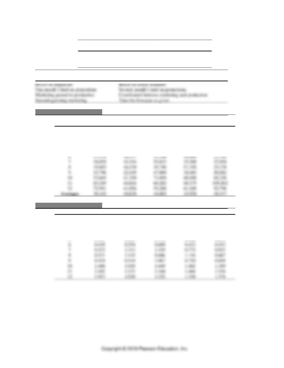
Board 2
Current Forecasting System
Proposed Forecasting System
Based on shipments
Based on actual demands
One month’s lead on promotions
Several month’s lead on promotions
Marketing passed to production
Coordinated between marketing and production
Second-guessing marketing
Take the forecasts as given
EXHIBIT TN.1
Actual Bow Rake Demands and Forecast
Actual Demands
Month
Year 1
Year 2
Year 3
Year 4
Forecast
1
55,220
39,875
32,180
62,377
70,203
2
57,350
64,128
38,600
66,501
72,911
3
15,445
47,653
25,020
31,404
19,636
4
27,776
43,050
51,300
36,504
35,312
5
21,408
39,359
31,790
16,888
27,217
6
17,118
10,317
32,100
18,909
21,763
7
18,028
45,194
59,832
35,500
22,920
8
19,883
46,530
30,740
51,250
25,278
9
15,796
22,105
47,800
34,443
20,082
10
53,665
41,350
73,890
68,088
68,226
11
83,269
46,024
60,202
68,175
105,862
12
72,991
41,856
55,200
61,100
92,796
Averages
38,162
40,620
44,805
45,928
48,517
EXHIBIT TN.2
Seasonal Factors
Month
Year 1
Year 2
Year 3
Year 4
Average
1
1.447
0.982
0.718
1.358
1.126
2
1.503
1.579
0.862
1.448
1.348
3
0.405
1.173
0.558
0.684
0.705
4
0.728
1.060
1.145
0.795
0.932
5
0.561
0.969
0.710
0.368
0.652
6
0.449
0.254
0.694
0.412
0.452
7
0.472
1.113
1.335
0.773
0.923
8
0.521
1.145
0.686
1.116
0.867
9
0.414
0.544
1.067
0.750
0.694
10
1.406
1.018
1.649
1.482
1.389
11
2.182
1.133
1.344
1.484
1.536
12
1.913
1.030
1.232
1.330
1.376
Forecasting ⚫ CHAPTER 8 ⚫
8-51
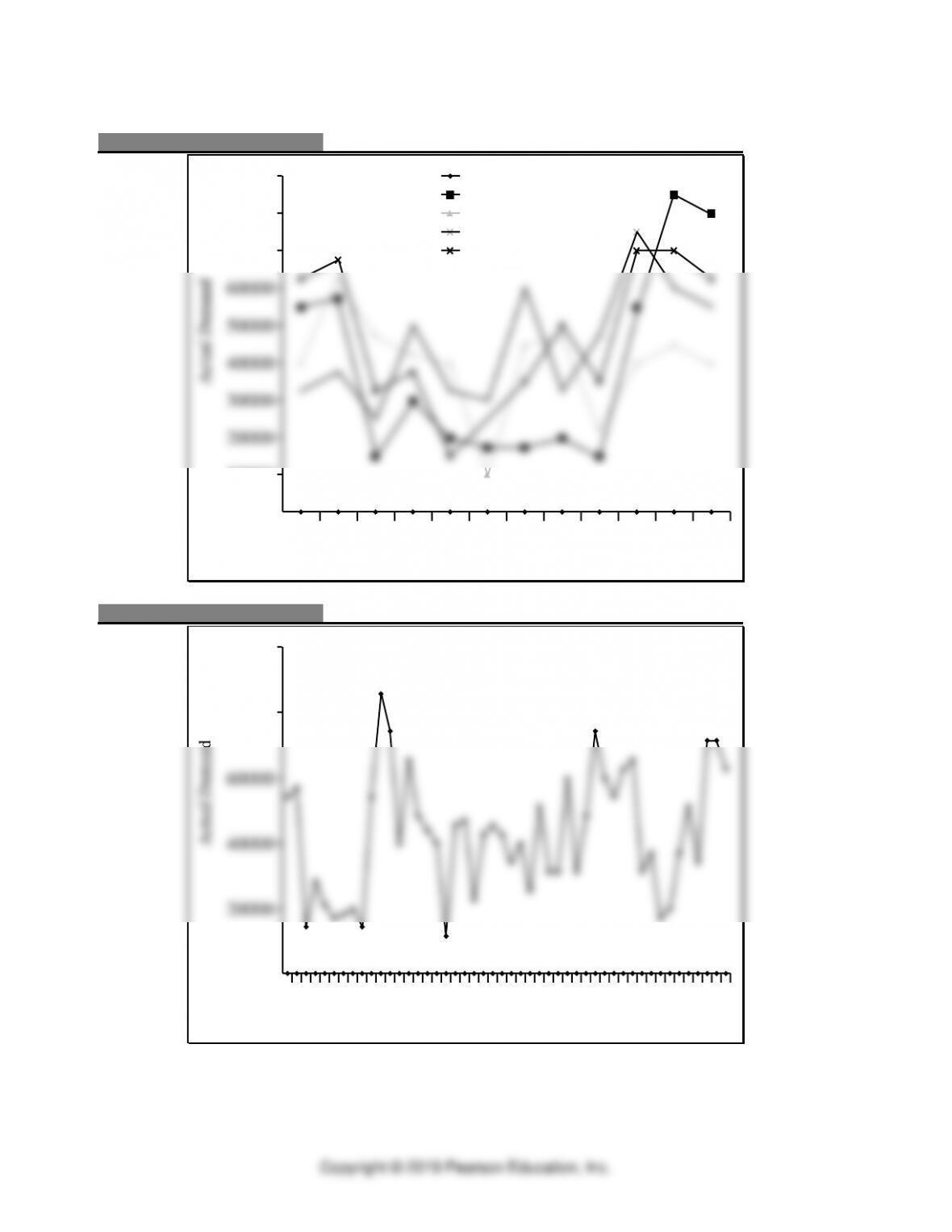
EXHIBIT TN.3
Monthly Demands
70000
60000
50000
40000
30000
20000
10000
2 4 6 8 10
Months
90000
80000
1 3 5 7 9 12
11
Year 1
Year 2
Year 3
Year 4
EXHIBIT TN.4
Four-Year Plot
60000
40000
20000
100000
80000

PART 2 Managing Customer Demand
8-52
EXPERIENTIAL LEARNING EXERCISE ONE
Forecasting a Vital Energy Statistic
Complete data set including 5-period holdout sample (April 01, 2011 – April 29, 2011)
Quarter 2
2010
Quarter 3
2010
Quarter 4
2010
Quarter 1
2011
Quarter 2
2011
Time Period
Data
Time Period
Data
Time Period
Data
Time Period
Data
Time Period
Data
Apr 02, 2010
1160
Jul 02, 2010
1116
Oct 01, 2010
1073
Dec 31, 2010
994
Apr 01, 2011
771
Apr 09, 2010
779
Jul 09, 2010
1328
Oct 08, 2010
857
Jan 07, 2011
1307
Apr 08, 2011
709
Apr 16, 2010
1134
Jul 16, 2010
1183
Oct 15, 2010
1197
Jan 14, 2011
997
Apr 15, 2011
562
Apr 23, 2010
1275
Jul 23, 2010
1219
Oct 22, 2010
718
Jan 21, 2011
1082
Apr 22, 2011
1154
Apr 30, 2010
1355
Jul 30, 2010
1132
Oct 29, 2010
817
Jan 28, 2011
887
Apr 29, 2011
998
May 07, 2010
1513
Aug 06, 2010
1094
Nov 05, 2010
946
Feb 04, 2011
1067
May 14, 2010
1394
Aug 13, 2010
1040
Nov 12, 2010
725
Feb 11, 2011
890
May 21, 2010
1097
Aug 20, 2010
1053
Nov 19, 2010
748
Feb 18, 2011
865
May 28, 2010
1206
Aug 27, 2010
1232
Nov 26, 2010
1031
Feb 25, 2011
858
Jun 04, 2010
1264
Sep 03, 2010
1073
Dec 03, 2010
1061
Mar 04, 2011
814
Jun 11, 2010
1153
Sep 10, 2010
1329
Dec 10, 2010
1074
Mar 11, 2011
871
Jun 18, 2010
1424
Sep 17, 2010
1096
Dec 17, 2010
941
Mar 18, 2011
1255
Jun 25, 2010
1274
Sep 24, 2010
1125
Dec 24, 2010
994
Mar 25, 2011
980
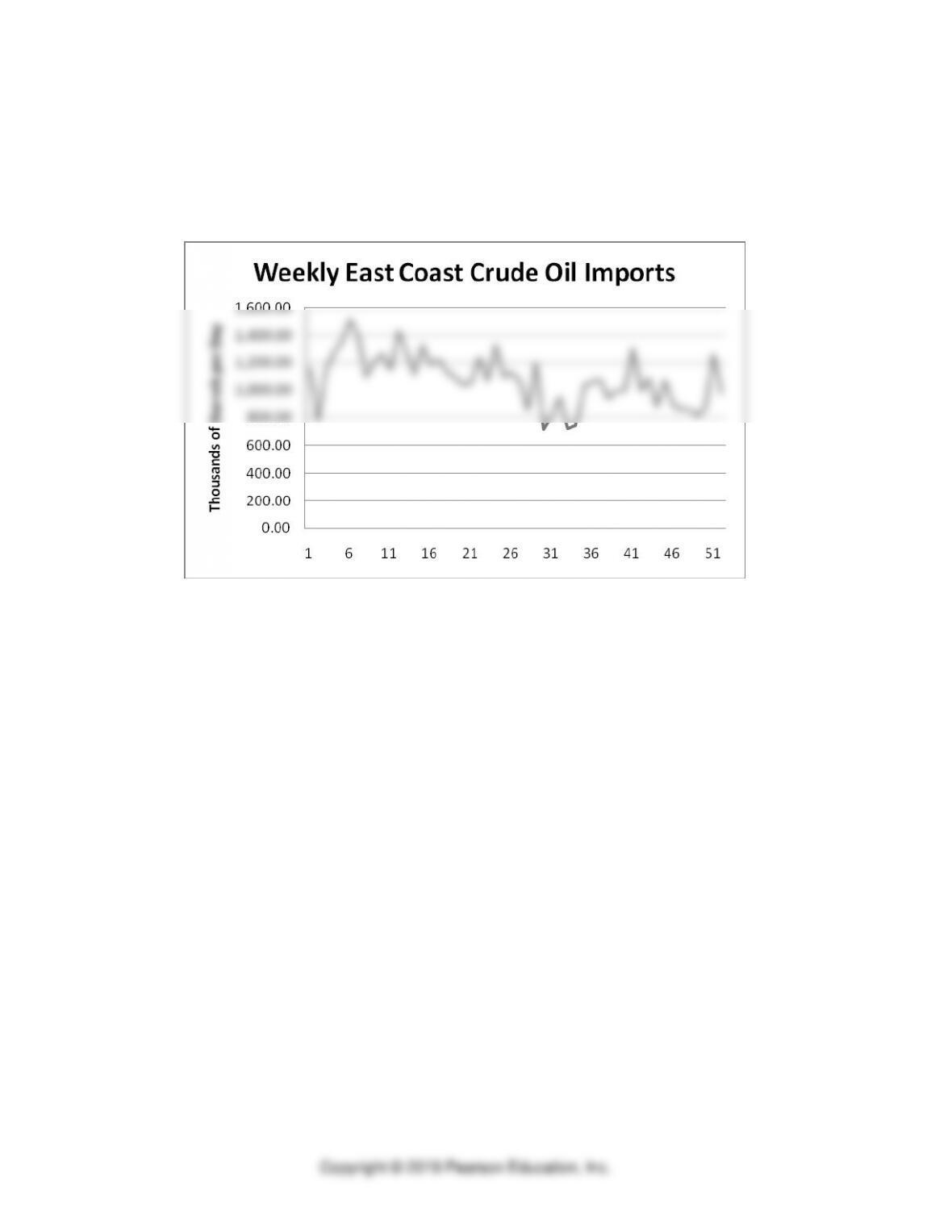
The Data Set:
Weekly East Coast Crude Oil Imports (in Thousand Barrels per Day)
Source:
The US Energy Information Administration
Excel File Name:
psw09.xls
Available from Web Page:
http://www.eia.gov/oil_gas/petroleum/data_publications/weekly_petroleum_status_report/wpsr.html
Source Web Site:
Energy Information Administration
For Help, Contact:
infoctr@eia.gov
(202) 586-8800
Forecasting ⚫ CHAPTER 8 ⚫
8-53
a. Use the Time Series Forecasting Solver of OM Explorer to develop initial forecasts for the
history file..
The time series plot shows the week-to-week variation in oil imports. A slight downward trend
but no obvious seasonality is evident.
The Time Series Forecasting Solver of OM Explorer provides calculation worksheets and results
for the each of the models suggested for this exercise.


