Unlock document.
This document is partially blurred.
Unlock all pages and 1 million more documents.
Get Access

Chapter
8
Forecasting
DISCUSSION QUESTIONS
1. a. There is no apparent trend in the data. The naïve forecast method, exponential
smoothing or the simple moving average would be appropriate for estimating the
average.
d. In the area of technological forecasting, qualitative methods of forecasting are best. One
2. What’s Happening? Our objective in writing this discussion question is to ensure students
recognize the difference between sales and demand. Demand forecasting techniques require
demand data. Michael is making the common mistake of using sales data as the basis for
demand forecasts. Sales are generally equal to the lesser of demand or inventory. Say that

PART 2 Managing Customer Demand
8-2
PROBLEMS
Causal Methods: Linear Regression
1. Garcia’s Garage
a. The results, using the Regression Analysis Solver of OM Explorer, are:
b. Forecasts
Y (Sep) = 42.464 + 2.452 (9) = 64.532 or 65
2. Hydrocarbon Processing Factory
Using the Regression Analysis Solver of OM Explorer, we get:
a. Relationship to forecast Y from X
Y = 0.888 + 0.622 X
b. Strength of relationship between Y and X is moderate as indicated by

Forecasting ⚫ CHAPTER 8 ⚫
8-3
3. Ohio Swiss Milk
The results from the Regression Analysis Solver are:
b. R2 = 0.888
R = −0.942 indicates a fairly strong negative relationship. Increases in costs explain
89% of the decreases in gallons sold
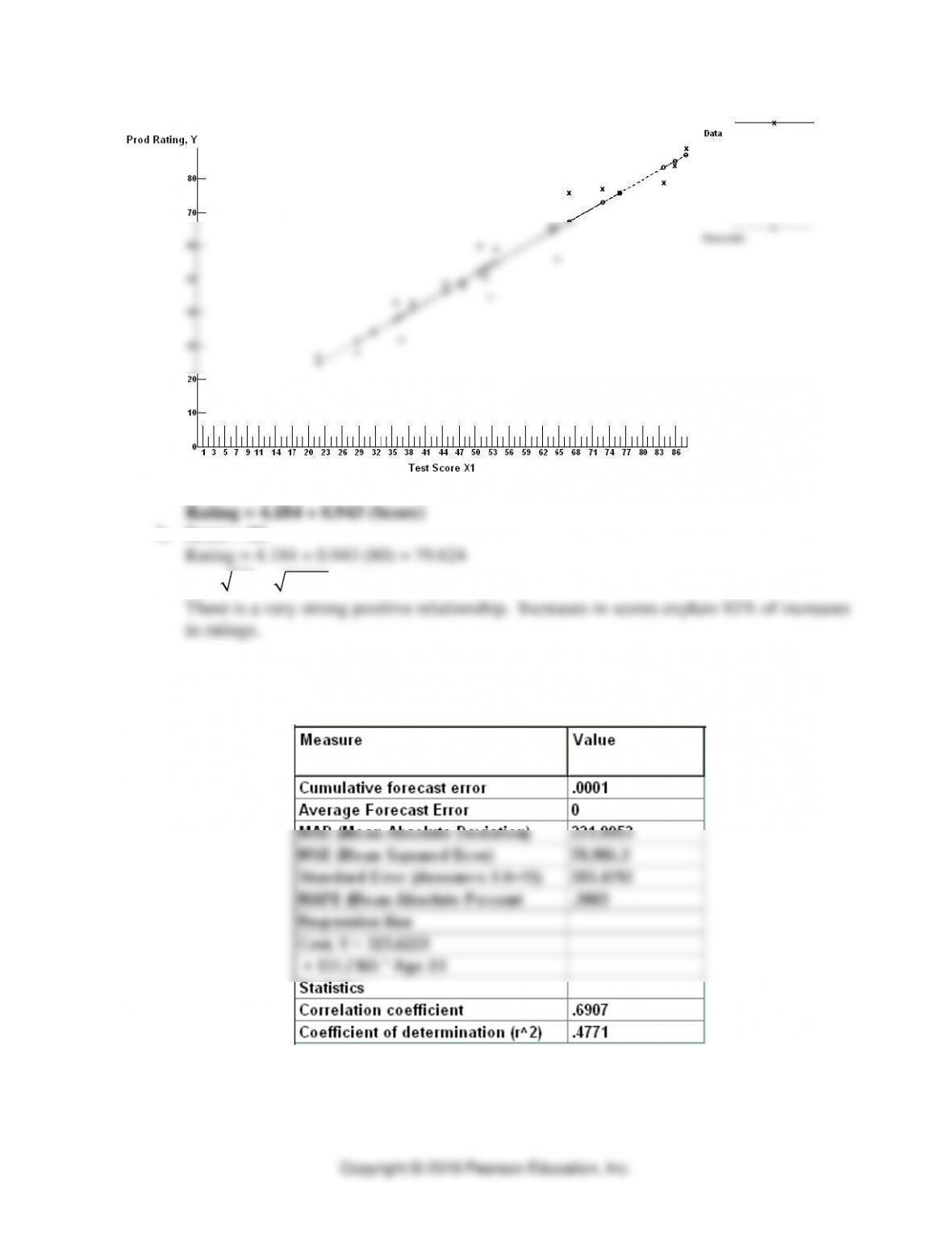
4. Manufacturing firm skills test
The results from the Least Square Linear Regression module of POM for Windows are:
PART 2 Managing Customer Demand
8-4
a. From the output, the relationship is
b. Score = 80
c.
20.934 0.966RR= = =
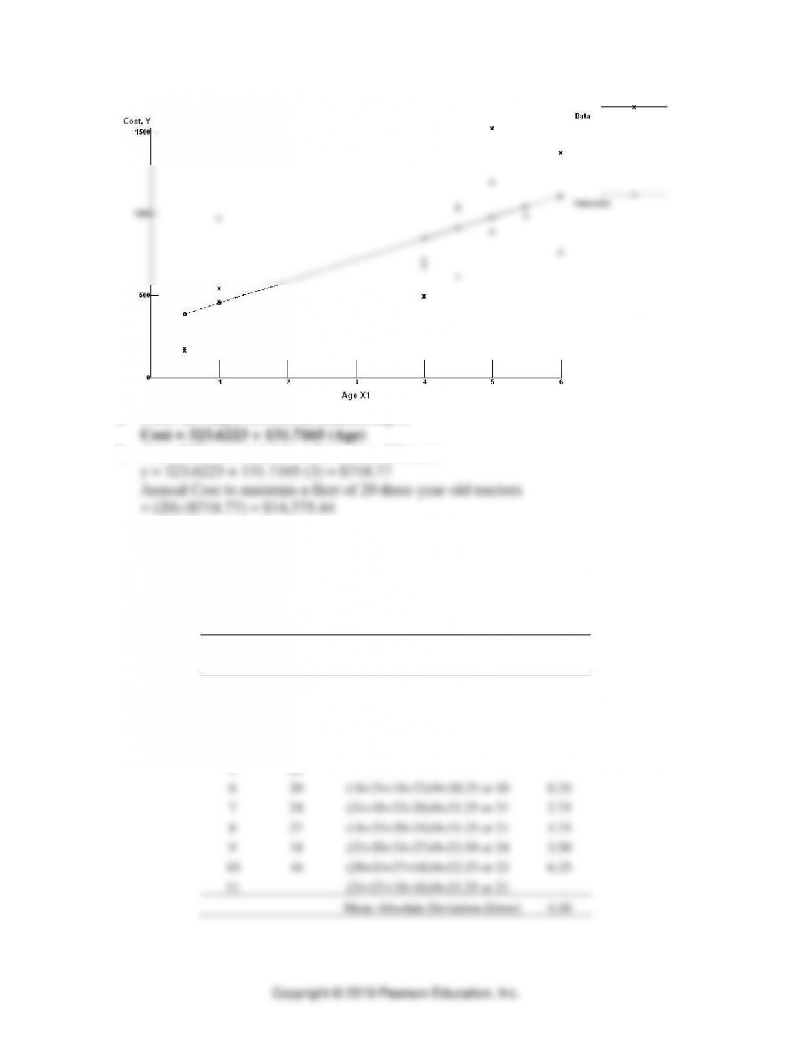
5. Materials handing
The results from the POM for Windows’ least squares-linear regression module are:
Forecasting ⚫ CHAPTER 8 ⚫
8-5
a. From the output shown, the relationship is
b. Annual Cost to maintain a three-year old tractor
Time-Series Methods
6. Handy Man Rentals
a. The forecast for week 11 is 21 rentals
b. The mean absolute deviation is 4.1 rentals
Week
Actual
Rentals
Four-Month Simple Moving
Average Forecast
Absolute
Error
1
15
2
16
3
24
4
18
5
23
6
20
(16+24+18+23)/4=20.25 or 20
0.25
7
24
(24+18+23+20)/4=21.25 or 21
2.75
8
27
(18+23+20+24)/4=21.25 or 21
5.75
9
18
(23+20+24+27)/4=23.50 or 24
5.50
10
16
(20+24+27+18)/4=22.25 or 22
6.25
11
(24+27+18+16)/4=21.25 or 21
Mean Absolute Deviation (Error)
4.10
7. Computer Success
PART 2 Managing Customer Demand
8-6
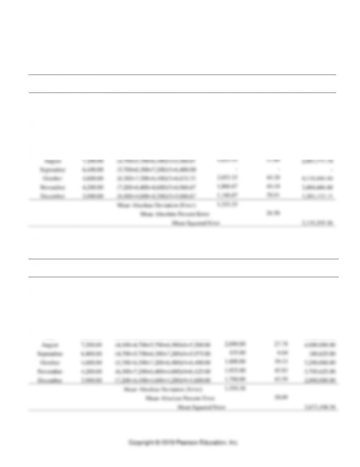
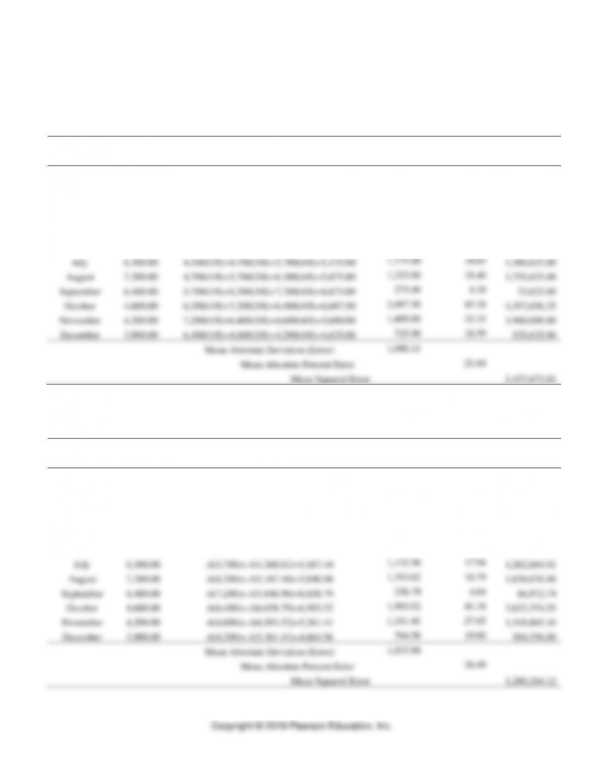
a. The three-month moving average forecast and forecast error calculations are shown in
the table below.
Month
Actual
Sales ($)
Three-Month Simple Moving
Average Forecast
Absolute
Error
Absolute
Percent Error
Squared Error
January
3,000.00
February
3,400.00
March
3,700.00
April
4,100.00
May
4,700.00
(3,400+3,700+4,100)/3=3,733.33
966.67
20.57
934,444.44
June
5,700.00
(3,700+4,100+4,700)/3=4,166.67
1,533.33
26.90
2,351,111.11
July
6,300.00
(4,100+4,700+5,700)/3=4,833.33
1,466.67
23.28
2,151,111.11
August
7,200.00
(4,700+5,700+6,300)/3=5,566.67
1,633.33
22.69
2,667,777.78
September
6,400.00
(5,700+6,300+7,200)/3=6,400.00
-
-
-
October
4,600.00
(6,300+7,200+6,400)/3=6,633.33
2,033.33
44.20
4,134,444.44
November
4,200.00
(7,200+6,400+4,600)/3=6,066.67
1,866.67
44.44
3,484,444.44
December
3,900.00
(6,400+4,600+4,200)/3=5,066.67
1,166.67
29.91
1,361,111.11
Mean Absolute Deviation (Error)
1,333.33
Mean Absolute Percent Error
26.50
Mean Squared Error
2,135,555.56
b. The four-month moving average forecast and forecast error calculations are shown in
the table below.
Month
Actual Sales
($)
Four-Month Simple Moving Average
Forecast
Absolute
Error
Absolute
Percent Error
Squared Error
January
3,000.00
February
3,400.00
March
3,700.00
April
4,100.00
May
4,700.00
(3,000+3,400+3,700+4,100)/4=3,550.00
1,150.00
24.47
1,322,500.00
June
5,700.00
(3,400+3,700+4,100+4,700)/4=3,975.00
1,725.00
30.26
2,975,625.00
July
6,300.00
(3,700+4,100+4,700+5,700)/4=4,550.00
1,750.00
27.78
3,062,500.00
August
7,200.00
(4,100+4,700+5,700+6,300)/4=5,200.00
2,000.00
27.78
4,000,000.00
September
6,400.00
(4,700+5,700+6,300+7,200)/4=5,975.00
425.00
6.64
180,625.00
October
4,600.00
(5,700+6,300+7,200+6,400)/4=6,400.00
1,800.00
39.13
3,240,000.00
November
4,200.00
(6,300+7,200+6,400+4,600)/4=6,125.00
1,925.00
45.83
3,705,625.00
December
3,900.00
(7,200+6,400+4,600+4,200)/4=5,600.00
1,700.00
43.59
2,890,000.00
Mean Absolute Deviation (Error)
1,559.38
Mean Absolute Percent Error
30.69
Mean Squared Error
2,672,109.38
Forecasting ⚫ CHAPTER 8 ⚫
8-7
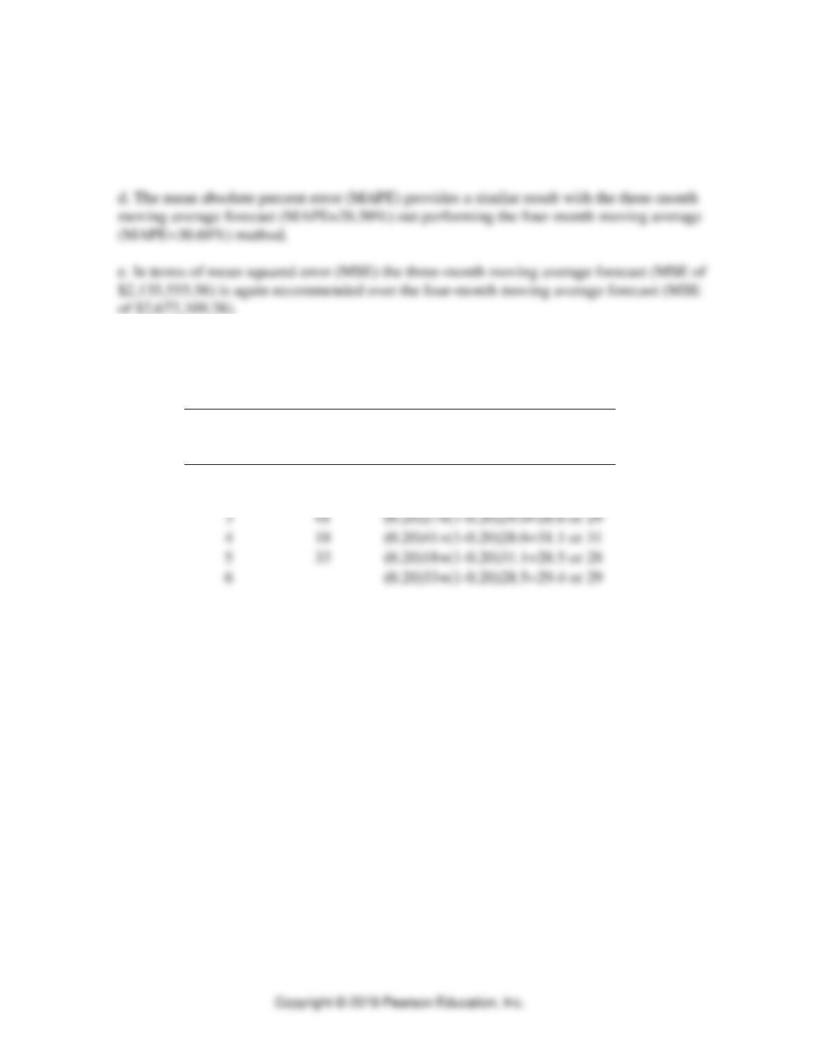
c. As seen in the tables above, the mean absolute deviation (MAD) of the three-month
moving average forecast is $1,333.33 and the four-month moving average forecast has a
somewhat greater MAD of $1,559.38. Thus, the three-month moving average method is
recommended.
8. Bradley’s Copiers
The exponentially smoothed forecast (α=0.20) for week 6 is 29 service calls
Week
Actual
Service
Calls
Exponentially Smoothed Forecast
(α=0.20)
1
29
29
2
27
(0.20)29+(1-0.20)29.0=29.0 or 29
3
41
(0.20)27+(1-0.20)29.0=28.6 or 29
4
18
(0.20)41+(1-0.20)28.6=31.1 or 31
5
33
(0.20)18+(1-0.20)31.1=28.5 or 28
6
(0.20)33+(1-0.20)28.5=29.4 or 29
PART 2 Managing Customer Demand
8-8
9. Computer Success (part 2)
a. The three-month weighted moving average forecast and forecast error calculations are
shown in the table below.
Month
Actual
Sales ($)
Three-Month Weighted Moving Average
Forecast
Absolute
Error
Absolute
Percent Error
Squared Error
January
3,000.00
February
3,400.00
March
3,700.00
April
4,100.00
3,000(1/8)+3,400(3/8)+3,700(4/8)=3,500.00
600.00
14.63
360,000.00
May
4,700.00
3,400(1/8)+3,700(3/8)+4,100(4/8)=3,862.50
837.50
17.82
701,406.25
June
5,700.00
3,700(1/8)+4,100(3/8)+4,700(4/8)=4,350.00
1,350.00
23.68
1,822,500.00
July
6,300.00
4,100(1/8)+4,700(3/8)+5,700(4/8)=5,125.00
1,175.00
18.65
1,380,625.00
August
7,200.00
4,700(1/8)+5,700(3/8)+6,300(4/8)=5,875.00
1,325.00
18.40
1,755,625.00
September
6,400.00
5,700(1/8)+6,300(3/8)+7,200(4/8)=6,675.00
275.00
4.30
75,625.00
October
4,600.00
6,300(1/8)+7,200(3/8)+6,400(4/8)=6,687.50
2,087.50
45.38
4,357,656.25
November
4,200.00
7,200(1/8)+6,400(3/8)+4,600(4/8)=5,600.00
1,400.00
33.33
1,960,000.00
December
3,900.00
6,400(1/8)+4,600(3/8)+4,200(4/8)=4,625.00
725.00
18.59
525,625.00
Mean Absolute Deviation (Error)
1,086.11
Mean Absolute Percent Error
21.64
Mean Squared Error
1,437,673.61
b. The exponential smoothing forecast (α=0.6) and forecast error calculations are shown in
the table below.
Month
Actual
Sales ($)
Exponentially Smoothed Forecast (α=0.60)
Absolute
Error
Absolute
Percent Error
Squared Error
January
3,000.00
3,200.00
February
3,400.00
.6(3,000)+.4(3,200.00)=3,080.00
March
3,700.00
.6(3,400)+.4(3,080.00)=3,272.00
April
4,100.00
.6(3,700)+.4(3,272.00)=3,528.80
571.20
13.93
326,269.44
May
4,700.00
.6(4,100)+.4(3,528.80)=3,871.52
828.48
17.63
686,379.11
June
5,700.00
.6(4,700)+.4(3,871.52)=4,368.61
1,331.39
23.36
1,772,604.66
July
6,300.00
.6(5,700)+.4(4,368.61)=5,167.44
1,132.56
17.98
1,282,684.91
August
7,200.00
.6(6,300)+.4(5,167.44)=5,846.98
1,353.02
18.79
1,830,670.48
September
6,400.00
.6(7,200)+.4(5,846.98)=6,658.79
258.79
4.04
66,972.74
October
4,600.00
.6(6,400)+.4(6,658.79)=6,503.52
1,903.52
41.38
3,623,374.55
November
4,200.00
.6(4,600)+.4(6,503.52)=5,361.41
1,161.41
27.65
1,348,865.16
December
3,900.00
.6(4,200)+.4(5,361.41)=4,664.56
764.56
19.60
584,556.00
Mean Absolute Deviation (Error)
1,033.88
Mean Absolute Percent Error
20.49
Mean Squared Error
1,280,264.12
Forecasting ⚫ CHAPTER 8 ⚫
8-9
c. As seen in the tables above, the mean absolute deviation (MAD) of the exponential
smoothing forecast is $1,033.88 and the three-month weighted moving average forecast has
a somewhat greater MAD of $1,086.11. Thus, the exponential smoothing method is
recommended.
10. Convenience Store
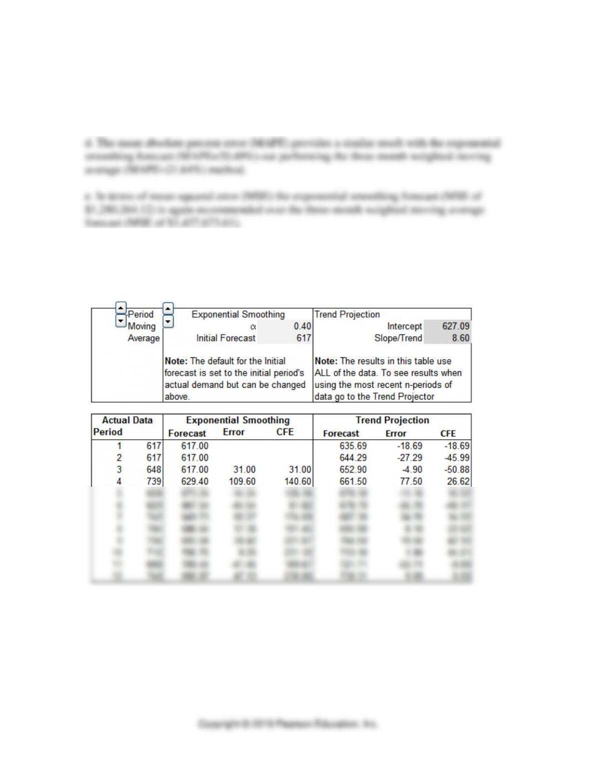
The worksheet calculations from the Time Series Forecasting Solver of OM Explorer for
both Exponential Smoothing and Trend Projection with Regression follow:
PART 2 Managing Customer Demand
8-10
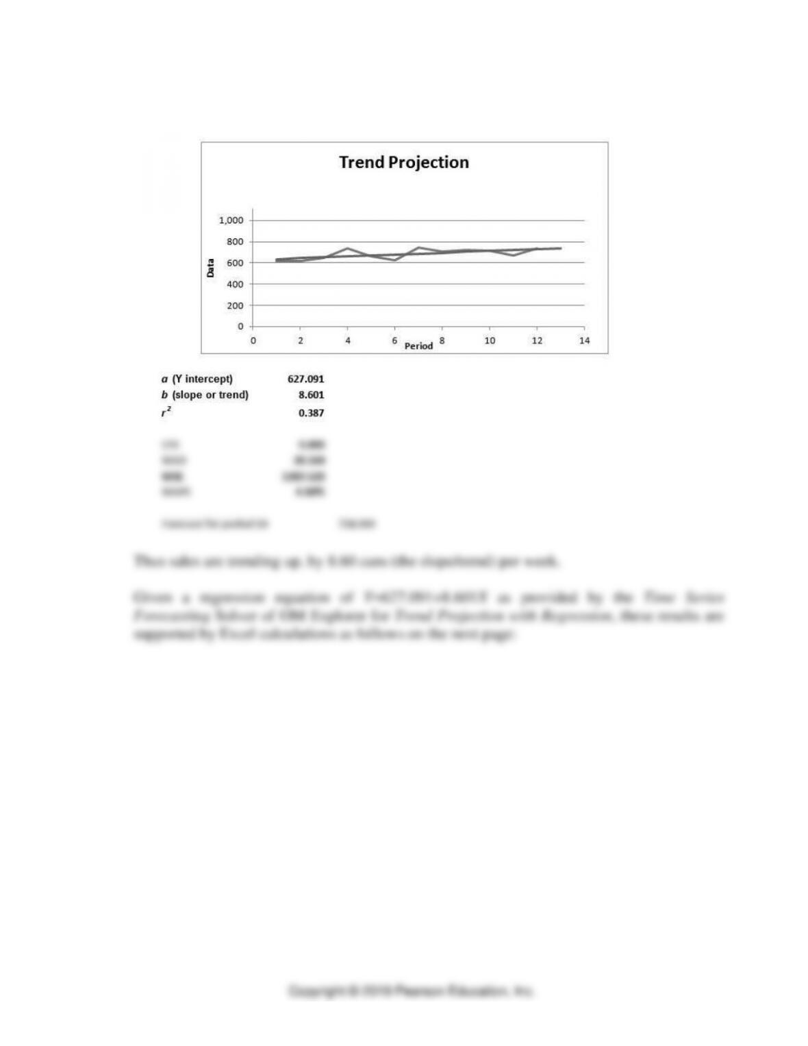
The results from the Time Series Forecasting Solver of OM Explorer for Trend Projection
with Regression:
Forecasting ⚫ CHAPTER 8 ⚫
8-11
Trend Projection with Regression
Week
(t)
Sales
Forecast
Error
Absolute
Error
Squared
Error
Absolute
Percent Error
1
617
635.7
-18.7
18.69
349.37
3.03
2
617
644.3
-27.3
27.29
744.90
4.42
3
648
652.9
-4.9
4.89
23.95
0.76
4
739
661.5
77.5
77.50
6006.93
10.49
5
659
670.1
-11.1
11.10
123.14
1.68
6
623
678.7
-55.7
55.70
3102.31
8.94
7
742
687.3
54.7
54.70
2992.11
7.37
8
704
695.9
8.1
8.10
65.59
1.15
9
724
704.5
19.5
19.50
380.15
2.69
10
715
713.1
1.9
1.90
3.59
0.27
11
668
721.7
-53.7
53.71
2884.27
8.04
12
740
730.3
9.7
9.69
93.96
1.31
Forecast
738.9
CFE
0.0
MAD
28.56
MSE
1397.52
MAPE
4.18
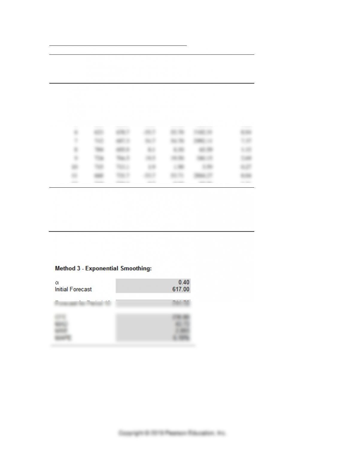
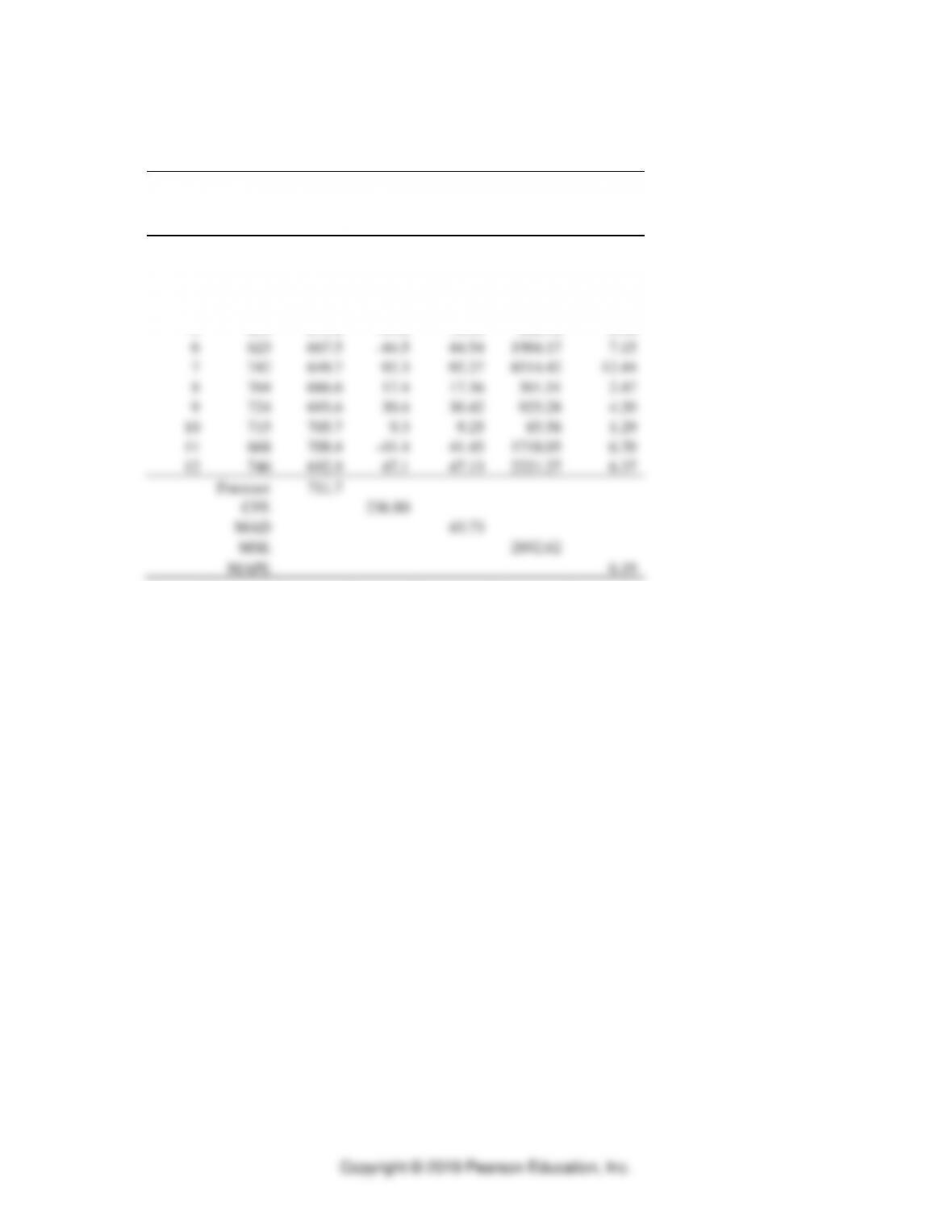
The results from the Time Series Forecasting Solver of OM Explorer for Exponential
Smoothing:
PART 2 Managing Customer Demand
8-12
These results are supported by Excel calculations as follows:
Exponential Smoothing
Week
(t)
Sales
Forecast
Error
Absolute
Error
Squared
Error
Absolute
Percent
Error
1
617
617.0
0.0
0.00
0.00
0.00
2
617
617.0
0.0
0.00
0.00
0.00
3
648
617.0
31.0
31.00
961.00
4.78
4
739
629.4
109.6
109.60
12012.16
14.83
5
659
673.2
-14.2
14.24
202.78
2.16
6
623
667.5
-44.5
44.54
1984.17
7.15
7
742
649.7
92.3
92.27
8514.42
12.44
8
704
686.6
17.4
17.36
301.51
2.47
9
724
693.6
30.4
30.42
925.28
4.20
10
715
705.7
9.3
9.25
85.58
1.29
11
668
709.4
-41.4
41.45
1718.05
6.20
12
740
692.9
47.1
47.13
2221.27
6.37
Forecast
711.7
CFE
236.80
MAD
43.73
MSE
2892.62
MAPE
6.19
Method Comparisons:
Trend Exponential
Projection Smoothing
MAD 28.56 43.73
MAPE 4.18 6.19
The Trend Projection with Regression method is superior for both MAD and MAPE. Thus, it appears that a
modest trend does exist. Trend component provided through regression analysis = 8.60 cans per week.
Forecasting ⚫ CHAPTER 8 ⚫
8-13
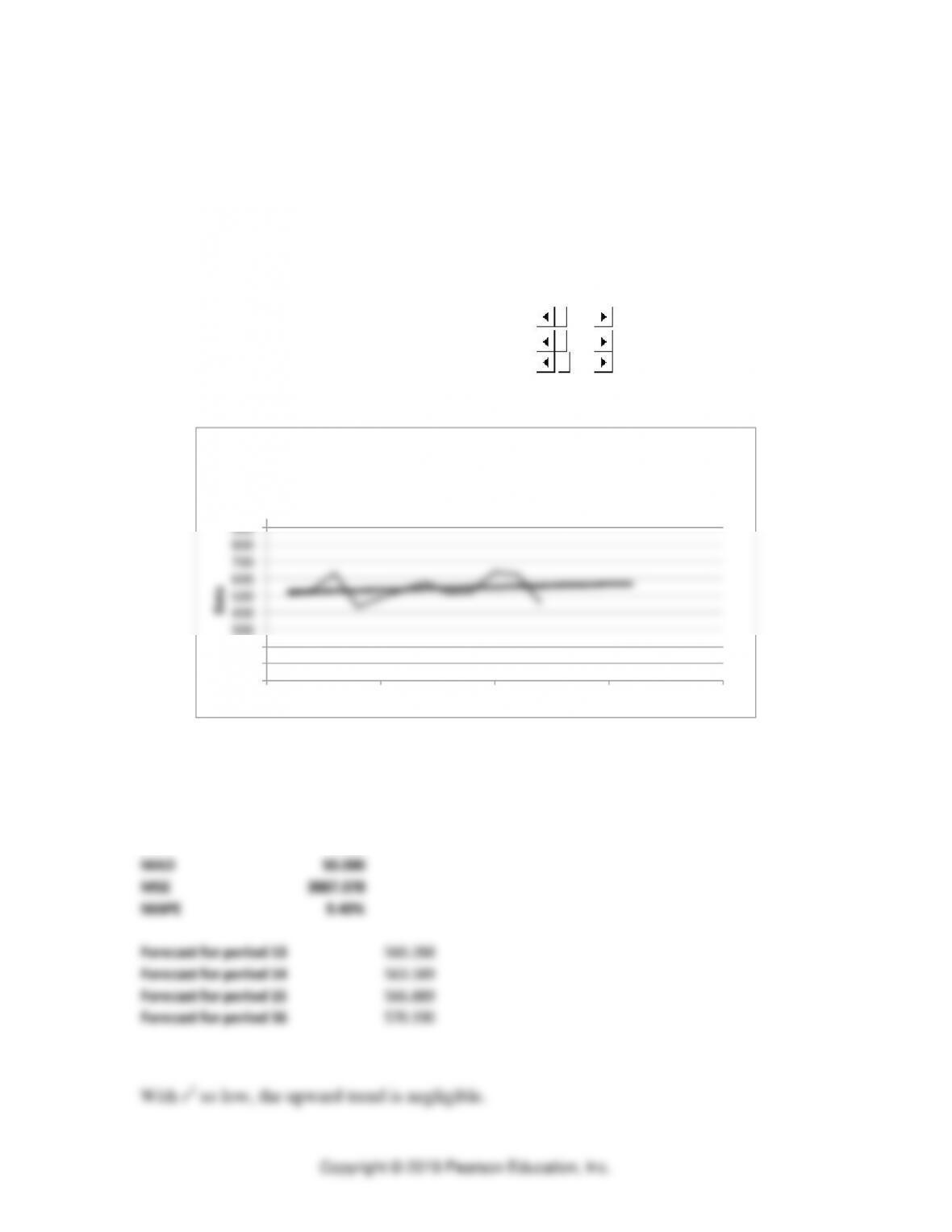
11. Community Federal
The results from the Time Series Forecasting Solver of OM Explorer for Trend Projection
with Regression are :
Results
Solver - Trend Projection with Regression
Regression begins in period 1check scrollbar
Error analysis begins in period 1
Number of future forecasts 4
a (Y intercept) 517.379
b (slope or trend) 3.301
r20.032
CFE 0.000
MAD 50.000
MSE 3887.978
MAPE 9.40%
Forecast for period 13 560.288
Forecast for period 14 563.589
Forecast for period 15 566.889
Forecast for period 16 570.190
0
100
200
300
400
500
600
700
800
900
0 5 10 15 20
Data
Period
Trend Projection
PART 2 Managing Customer Demand
8-14
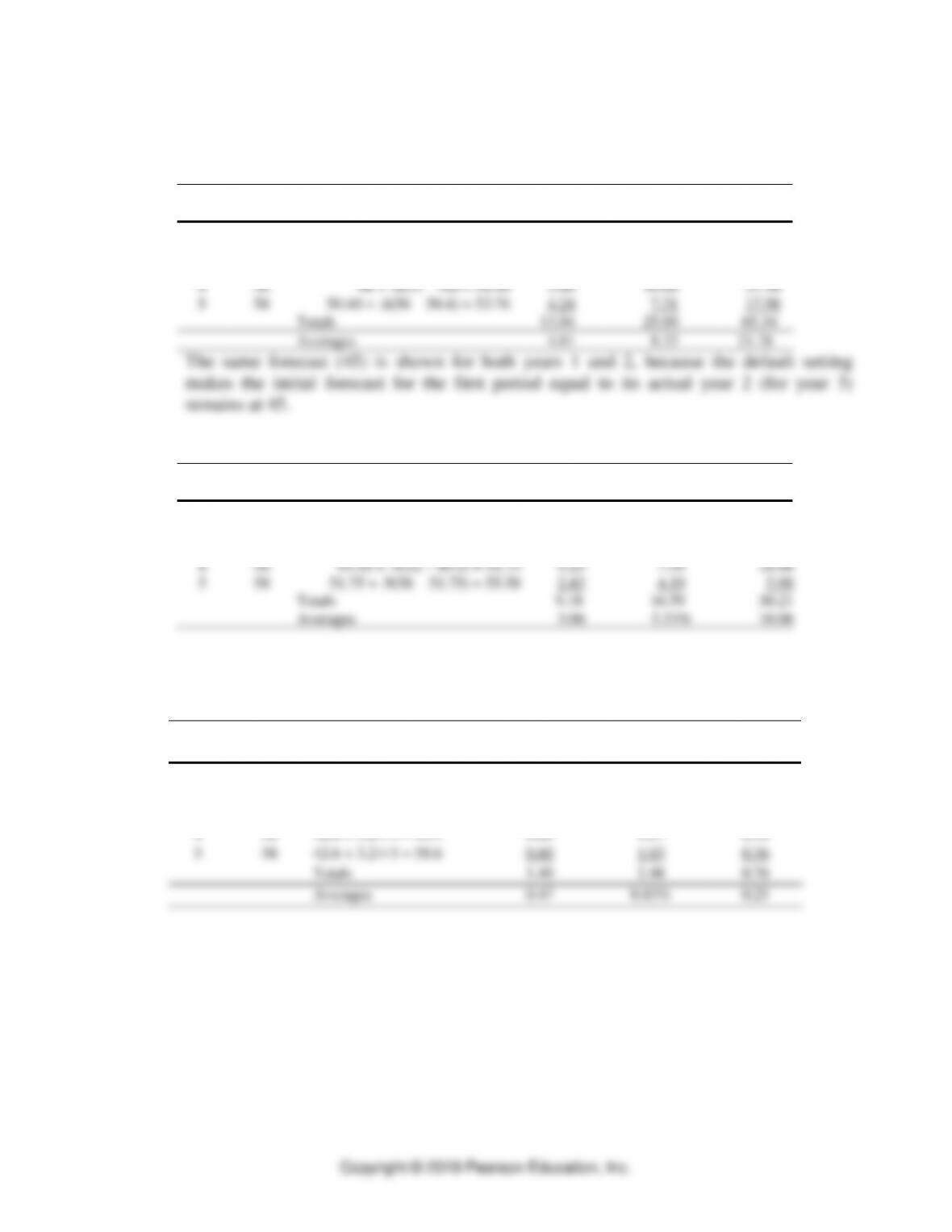
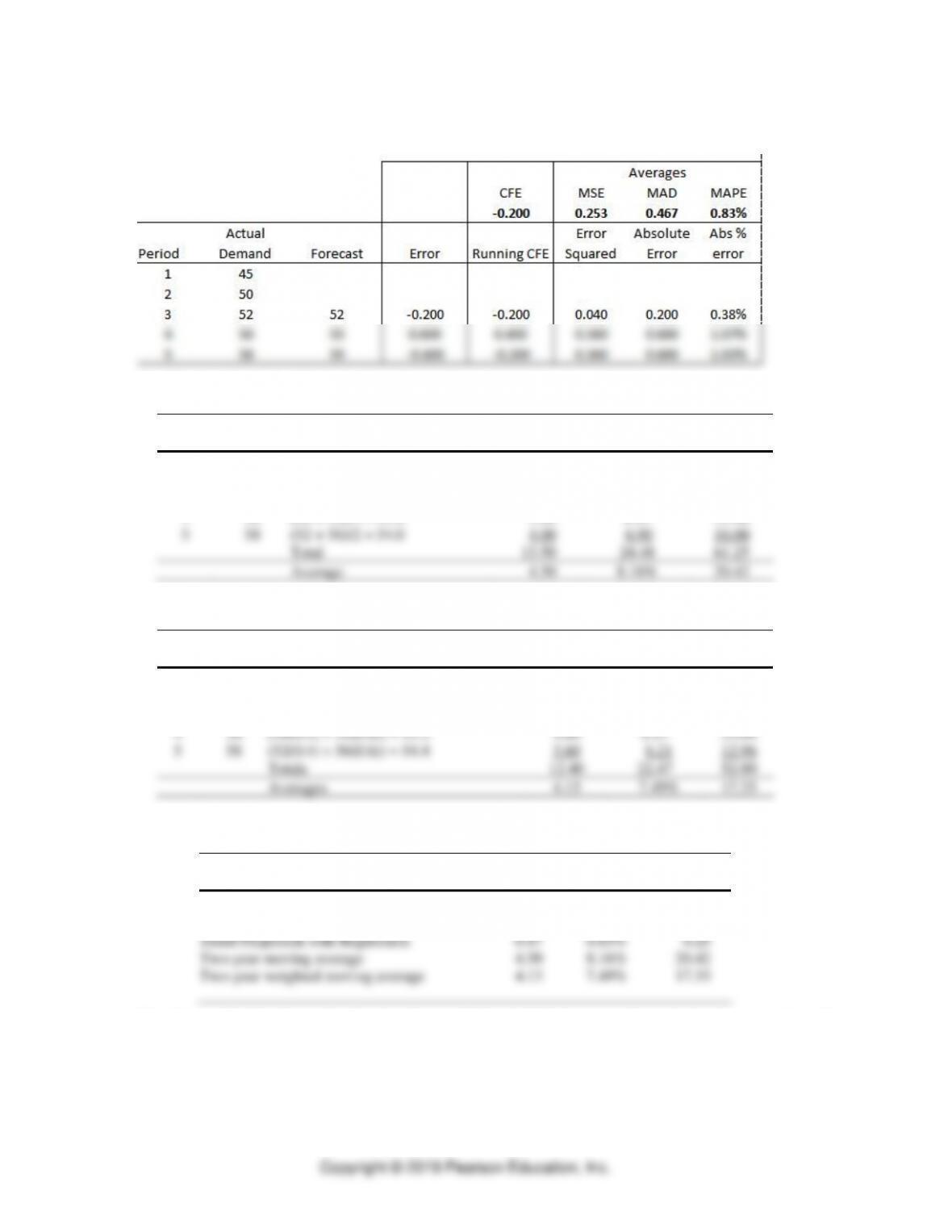
12. Heartville General Hospital
a. Exponential smoothing,
=0 6.
Year
Demand
Exponential Smoothing
Absolute
Absolute %
Square
Deviation
Deviation
Error
1
45
45
2
50
45 + .6(45 – 45) = 45
3
52
45 + .6(50 – 45) = 48
4.00
7.69
16.00
4
56
48 + .6(52 – 48) = 50.40
5.60
10.00
31.36
5
58
50.40 + .6(56 – 50.4) = 53.76
4.24
7.31
17.98
Totals
13.84
25.00
65.34
Averages
4.61
8.33
21.78
b. Exponential smoothing,
= 0.9
Year
Demand
Exponential Smoothing
Absolute
Absolute %
Squared
Deviation
Deviation
Error
1
45
45
2
50
45 + .9(45 – 45) = 45
3
52
45 + .9(50 – 45) = 49.50
2.50
4.81
6.25
4
56
49.50 + .9(52 – 49.5) = 51.75
4.25
7.59
18.06
5
58
51.75 + .9(56 – 51.75) = 55.58
2.43
4.19
5.90
Totals
9.18
16.59
30.21
Averages
3.06
5.53%
10.06
c. Trend Projection with Regression: model
Y X= +42 6 32. .
obtained from the Time Series
Forecasting Solver of OM Explorer for Trend Projection with Regression:
Year
Demand
Trend Projection
Absolute
Absolute %
Squared
Deviation
Deviation
Error
1
45
42.6 + 3.2
1 = 45.8
2
50
42.6 + 3.2
2 = 49.0
3
52
42.6 + 3.2
3 = 52.2
0.20
0.38
0.04
4
56
42.6 + 3.2
4 = 55.4
0.60
1.07
0.36
5
58
42.6 + 3.2
5 = 58.6
0.60
1.03
0.36
Totals
1.40
2.48
0.76
Averages
0.47
0.83%
0.25
Forecasting ⚫ CHAPTER 8 ⚫
8-15
These Excel computations are confirmed by the Trend Projection with Regression Solver of
OM Explorer:
d. Two-year moving average
Year
Demand
2-Year Moving
Absolute
Absolute %
Square
Average
Deviation
Deviation
Error
1
45
2
50
3
52
(45 + 50)/2 = 47.5
4.50
8.65
20.25
4
56
(50 + 52)/2 = 51.0
5.00
8.93
25.00
5
58
(52 + 56)/2 = 54.0
4.00
6.90
16.00
Total
13.50
24.48
61.25
Average
4.50
8.16%
20.42
e. Two-year weighted moving average
Year
Demand
2-Year Weighted
Absolute
Absolute %
Squared
Moving Average
Deviation
Deviation
Error
1
45
2
50
3
52
(45(0.4) + 50(0.6)) = 48.0
4.00
7.69
16.00
4
56
(50(0.4) + 52(0.6)) = 51.2
4.80
8.57
23.04
5
58
(52(0.4) + 56(0.6)) = 54.4
3.60
6.21
12.96
Totals
12.40
22.47
52.00
Averages
4.13
7.49%
17.33
f.-h. Comparison of the forecasting methodologies
Forecast
MAD
MAPE
MSE
Methodology
Exponential smoothing = .6
4.61
8.33%
21.78
Exponential smoothing = .9
3.06
5.53%
10.06
Trend Projection with Regression
0.47
0.83%
0.25
Two-year moving average
4.50
8.16%
20.42
Two-year weighted moving average
4.13
7.49%
17.33
The Trend Projection with Regression model methodology works best in this case for all
performance criteria.
PART 2 Managing Customer Demand
8-16
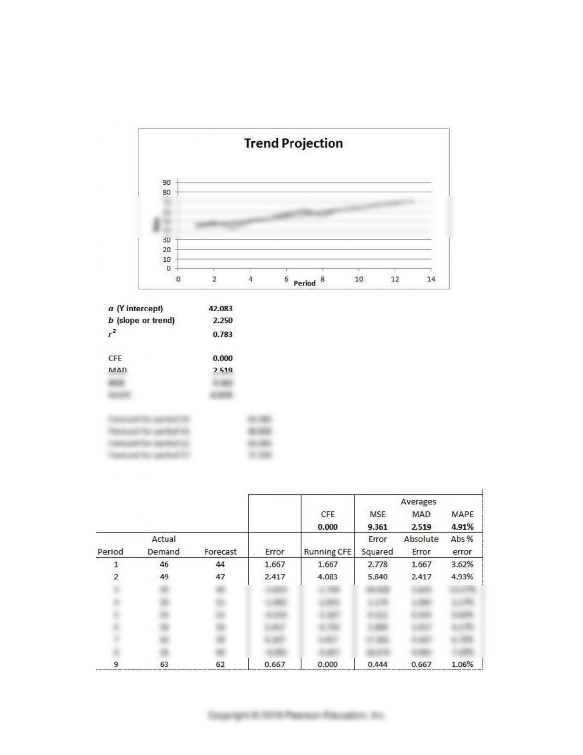
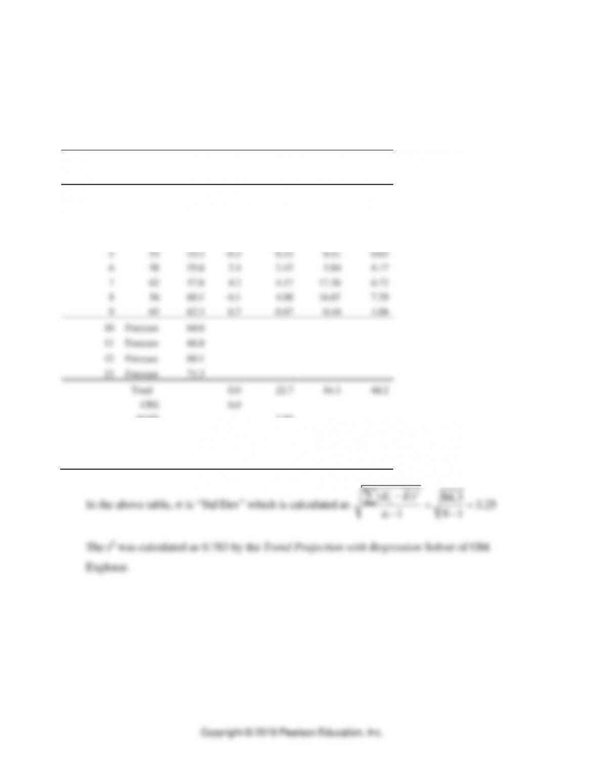
13. Calculator sales
The Trend Projection with Regression Solver of OM Explorer gives the following results:
Detailed analysis from the TPWorksheet is::
Forecasting ⚫ CHAPTER 8 ⚫
8-17
Trend Projection with Regression: model
42.083 2.250YX=+
obtained from the Time
Series Forecasting Solver of OM Explorer for Trend Projection with Regression. These
results are supported by Excel calculations as follows:
Trend Projection with Regression
Week (t)
Sales
Forecast
Error
Absolute
Error
Squared
Error
Absolute
Percent
Error
1
46
44.3
1.7
1.67
2.78
3.62
2
49
46.6
2.4
2.42
5.84
4.93
3
43
48.8
-5.8
5.83
34.02
13.57
4
50
51.1
-1.1
1.08
1.17
2.17
5
53
53.3
-0.3
0.33
0.11
0.63
6
58
55.6
2.4
2.42
5.84
4.17
7
62
57.8
4.2
4.17
17.36
6.72
8
56
60.1
-4.1
4.08
16.67
7.29
9
63
62.3
0.7
0.67
0.44
1.06
10
Forecast
64.6
11
Forecast
66.8
12
Forecast
69.1
13
Forecast
71.3
Total
0.0
22.7
84.3
44.2
CFE
0.0
MAD
2.52
MSE
9.36
MAPE
4.91
Std Dev
3.25
2
()
84.3 3.25
t
EE
−==
PART 2 Managing Customer Demand
8-18
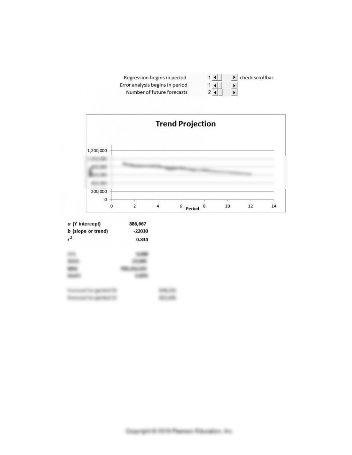
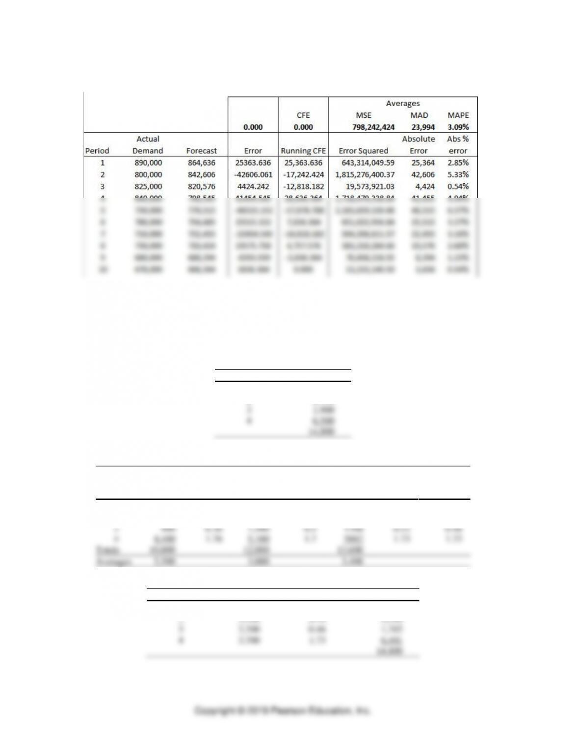
14. Krispee Crunchies
The Trend Projection with Regression Solver of OM Explorer gives the following results:
Forecasting ⚫ CHAPTER 8 ⚫
8-19
Detailed analysis from the TPWorksheet is:
If current conditions remain in place, the r2 of better than 80% provide some measure of
confidence that the downward trend (estimated at 22,030 boxes per month) will continue.
15. Forrest’s boxes of chocolates
a. One possible estimated forecast for Year 4:
Quarter
Forecast
1
3,700
2
2,700
3
1,900
4
6,500
14,800
b. Multiplicative seasonal method
Average
Seasonal
Seasonal
Seasonal
Seasonal
Quarter
Year 1
Factor
Year 2
Factor
Year 3
Factor
Factor
1
3,000
1.20
3,300
1.1
3502
1.03
1.11
2
1,700
0.68
2,100
0.7
2448
0.72
0.70
3
900
0.36
1,500
0.5
1768
0.52
0.46
4
4,400
1.76
5,100
1.7
5882
1.73
1.73
Totals
10,000
12,000
13,600
Averages
2,500
3,000
3,400
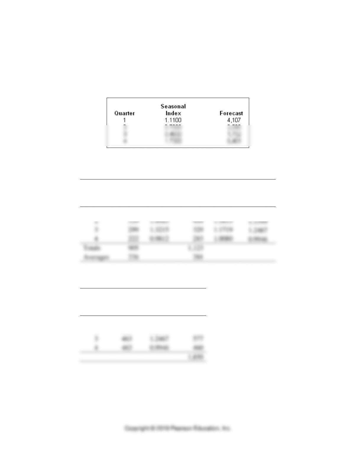
Forecast for year 4, 14,800. Average = 3,700.
Quarter
Average
Factor
Forecast
1
3,700
1.11
4,107
2
3,700
0.70
2,590
3
3,700
0.46
1,702
4
3,700
1.73
6,401
14,800
PART 2 Managing Customer Demand
8-20
This technique forecasts that the third-quarter sales will decrease compared to sales for
the third quarter of the third year. Betcha thought it would increase. Mamma always
said: “Life is full of surprises!”
Just to make sure, we find confirmation of our calculations using the Seasonal
Forecasting Solver of OM Explorer:
16. Alaina’s Garden Center
Quarter
Year 1
Seasonal
Factor
Year 2
Seasonal
Factor
Average
Seasonal
Factor
1
45
0.1989
67
0.2386
0.2188
2
339
1.4983
444
1.5815
1.5399
3
299
1.3215
329
1.1719
1.2467
4
222
0.9812
283
1.0080
0.9946
Totals
905
1,123
Averages
226
281
Forecast for year 3
1850
Quarter
Average
Forecast
Average
Seasonal
Factor
Year 3
Forecast
1
463
0.2188
101
2
463
1.5399
712
3
463
1.2467
577
4
463
0.9946
460
1,850


