Quality and Performance ⚫ CHAPTER 3 ⚫ 3–16
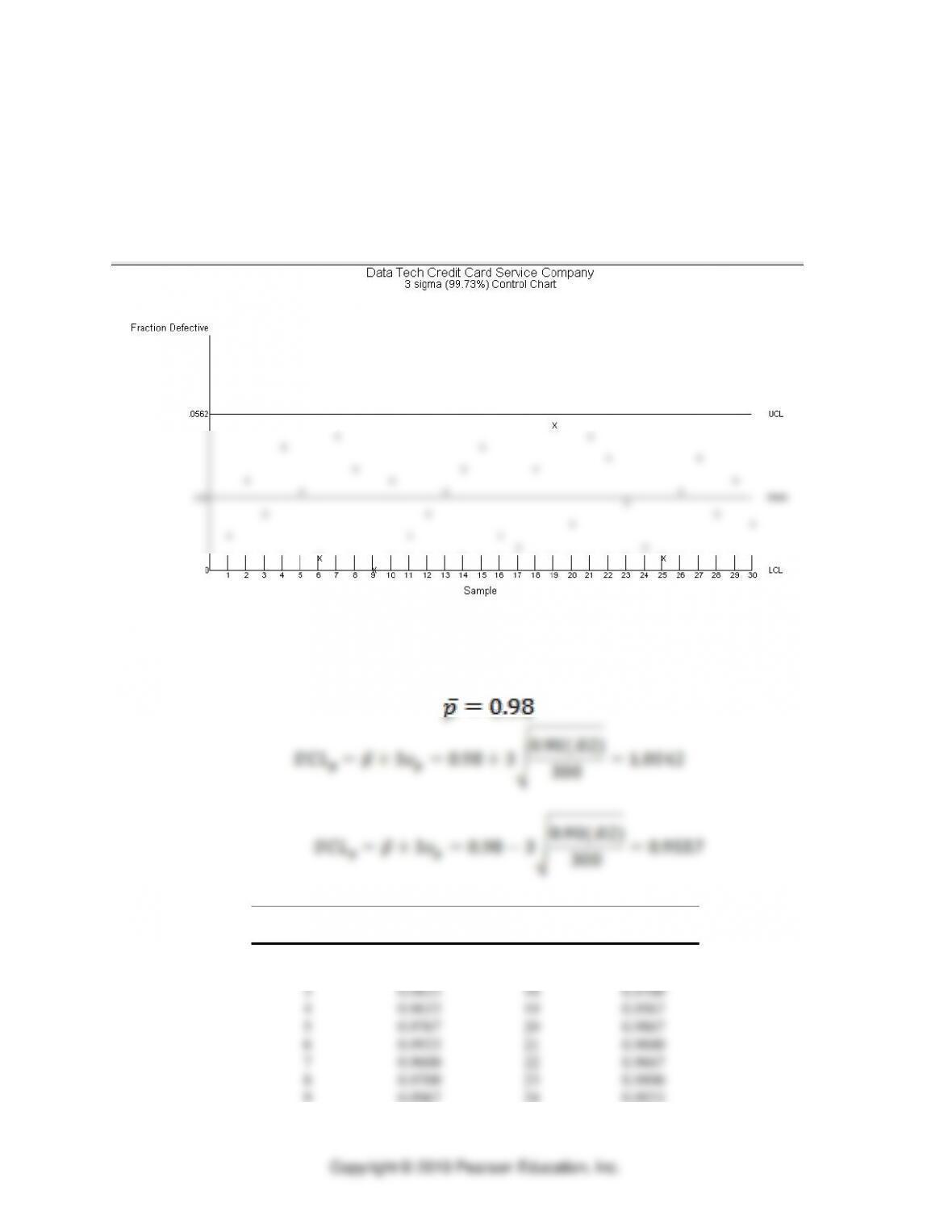
b. The POM for Windows graph below shows that all samples fall within the control
limits, but samples 11, 12, 13, 14, and 15 have an upward run and samples 21, 22, 23,
24, and 25 have a downward run. Because runs of 5 or more usually indicate
nonrandom behavior, we should investigate. We would like to avoid whatever was done
when samples 11–15 were taken and to repeat what was done during samples 21–25.
18. Red Baron Airlines
Management has set a high standard of 98 percent on-time performance, so the target
value for the chart’s central line is:
Proportion
Proportion
Sample
Defective
Sample
Defective
1
0.9900
16
0.9833
2
0.9733
17
0.9867
3
0.9833
18
0.9700
4
0.9633
19
0.9567
5
0.9767
20
0.9867
6
0.9933
21
0.9600
7
0.9600
22
0.9667
8
0.9700
23
0.9800
9
0.9967
24
0.9933
Quality and Performance ⚫ CHAPTER 3 ⚫ 3-17
10
0.9733
25
0.9967
11
0.9900
26
0.9733
12
0.9833
27
0.9867
13
0.9767
28
0.9833
14
0.9700
29
0.9733
15
0.9600
30
0.9933
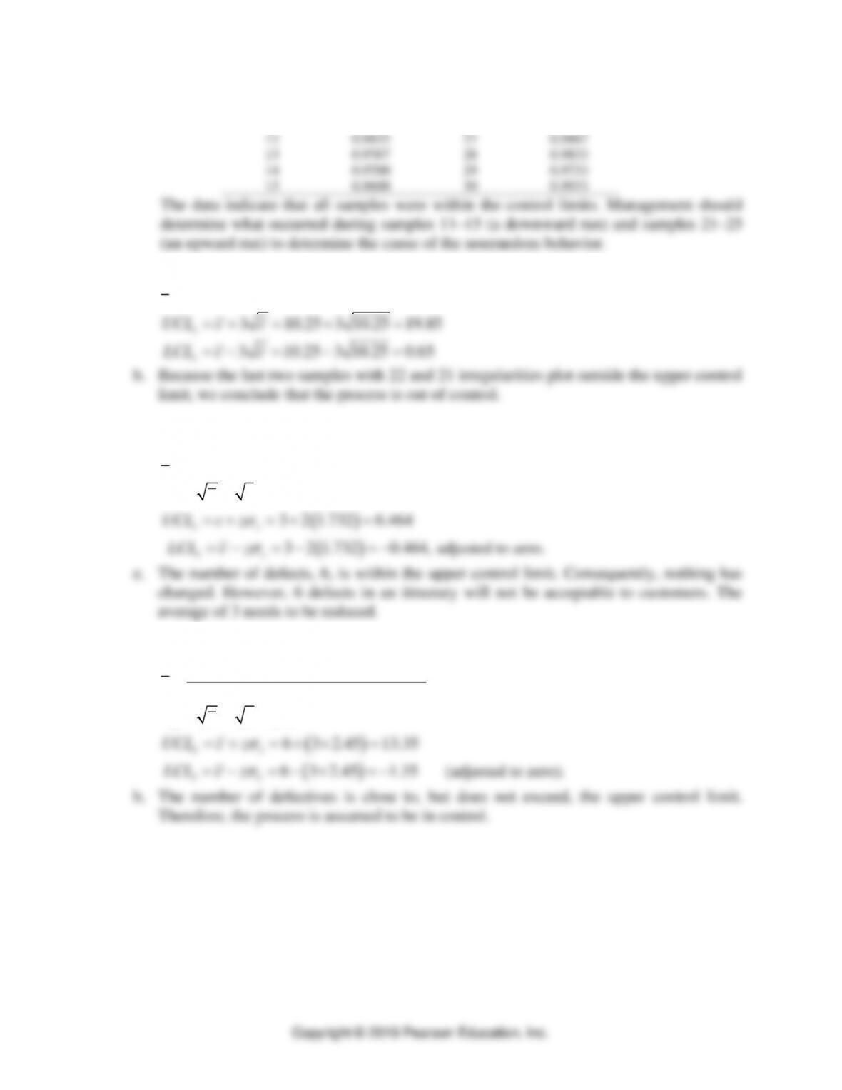
19. Textile manufacturer
a.
10.25c=
3 10.25 3 10.25 19.85
c
UCL c c= + = + =
3 10.25 3 10.25 0.65
c
LCL c c= − = − =
b. Because the last two samples with 22 and 21 irregularities plot outside the upper control
limit, we conclude that the process is out of control.
20. Travel agency
Because we cannot estimate how many errors were not made, we use a c-chart.
d.
c
= 3
3 1.732
cc
= = =
( )
3 2 1.732 6.464
cc
UCL c z
= + = + =
( )
3 2 1.732 0.464,
cc
LCL c z
= − = − = −
adjusted to zero.
e. The number of defects, 6, is within the upper control limit. Consequently, nothing has
changed. However, 6 defects in an itinerary will not be acceptable to customers. The
average of 3 needs to be reduced.
21. Jim’s Outfitters Inc.
a.
( )
8 0 7 12 5 10 2 4 6 6 6
10
c+ + + + + + + + +
==
6 2.45
cc
= = =
( )
6 3 2.45 13.35
cc
UCL c z
= + = + =
( )
6 3 2.45 1.35
cc
LCL c z
= − = − = −
(adjusted to zero).
b. The number of defectives is close to, but does not exceed, the upper control limit.
Therefore, the process is assumed to be in control.
Quality and Performance ⚫ CHAPTER 3 ⚫ 3–18
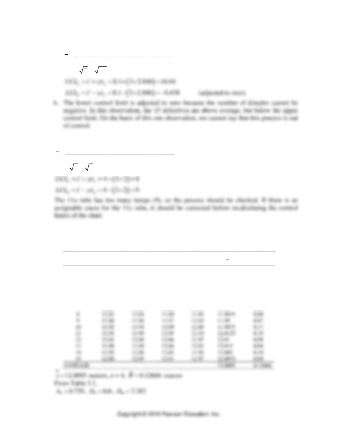
22. Big Black Bird
a.
( )
7 9 14 11 3 12 8 4 7 6 8.1
10
c+ + + + + + + + +
==
8.1 2.846
cc
= = =
( )
8.1 3 2.846 16.64
cc
UCL c z
= + = + =
( )
8.1 3 2.846 0.438
cc
LCL c z
= − = − = −
(adjusted to zero).
b. The lower control limit is adjusted to zero because the number of dimples cannot be
negative. In this observation, the 15 defectives are above average, but below the upper
control limit. On the basis of this one observation, we cannot say that this process is out
of control.
23. Webster, c-chart
( )
6 5 0 4 6 4 1 6 5 0 9 2 4
12
c+ + + + + + + + + + +
==
42
cc
= = =
( )
4 2 2 8
cc
UCL c z
= + = + =
( )
4 2 2 0
cc
LCL c z
= − = − =
The 11th tube has too many lumps (9), so the process should be checked. If there is an
assignable cause for the 11th tube, it should be corrected before recalculating the control
limits of the chart.
Process Capability
24. Sunny Soda, Inc.
Observation
Sample
1
2
3
4
x
R
1
12.00
11.97
12.10
12.08
12.0375
0.13
2
11.91
11.94
12.10
11.96
11.9775
0.19
3
11.89
12.02
11.97
11.99
11.9675
0.13
4
12.10
12.09
12.05
11.95
12.0475
0.15
5
12.08
11.92
12.12
12.05
12.0425
0.20
6
11.94
11.98
12.06
12.08
12.015
0.14
7
12.09
12.00
12.00
12.03
12.03
0.09
8
12.01
12.04
11.99
11.95
11.9975
0.09
9
12.00
11.96
11.97
12.03
11.99
0.07
10
11.92
11.94
12.09
12.00
11.9875
0.17
11
11.91
11.99
12.05
12.10
12.0125
0.19
12
12.01
12.00
12.06
11.97
12.01
0.09
13
11.98
11.99
12.06
12.03
12.015
0.08
14
12.02
12.00
12.05
11.95
12.005
0.10
15
12.00
12.05
12.01
11.97
12.0075
0.08
AVERAGE
12.0095
0.12666
12.0095x=
ounces, n = 4,
0.12666R=
ounces
From Table 3.1,
20.729A=
,
30.0D=
,
42.282D=
Quality and Performance ⚫ CHAPTER 3 ⚫ 3-19
Copyright © 2019 Pearson Education, Inc.
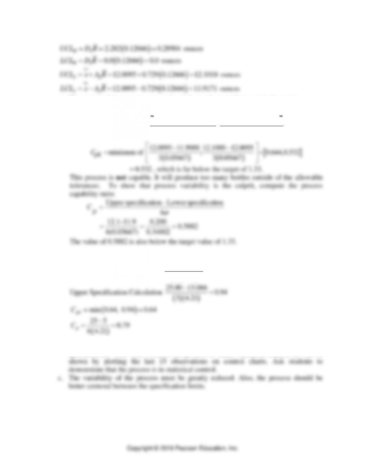
( )
42.282 0.12666 0.28904
R
UCL D R= = =
ounces
( )
30.0 0.12666 0.0
R
LCL D R= = =
ounces
( )
212.0095 0.729 0.12666 12.1018
x
UCL x A R= + = + =
ounces
( )
212.0095 0.729 0.12666 11.9171
x
LCL x A R= − = − =
ounces
a. The range and the process average for each sample are within statistical control.
b. The standard deviation of the data is 0.05667.
minimumof ;
33
x Lower specification Upper specification x
Cpk
−−
=
25. The Money Pit
a. Lower Specification Calculation
( )( )
13.066 5.00 0.64
3 4.21
−=
25.00 13.066 0.94
−=
( )
6 4.21
p
b. Because
p
C
and
pk
C
have values less than 1, the process is not capable of meeting
specifications. Yes, valid because the process is under statistical control, as can be
Quality and Performance ⚫ CHAPTER 3 ⚫ 3–20
26. Farley Manufacturing
Observation (millimeters)
Sample
1
2
3
4
5
6
7
8
1
9.100
8.900
8.800
9.200
8.100
6.900
9.300
9.100
2
7.600
8.000
9.000
10.100
7.900
9.000
8.000
8.800
3
8.200
9.100
8.200
8.700
9.000
7.000
8.800
10.800
4
8.200
8.300
7.900
7.500
8.900
7.800
10.100
7.700
5
10.000
8.100
8.900
9.000
9.300
9.000
8.700
10.000
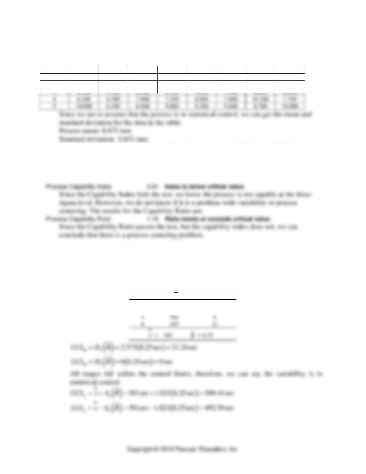
The critical value for the analysis is 1.0 for three-sigma quality. Using the OM Explorer
Solver for Process Capability, we get the following results:
Lower Spec Calculation
1.44
Upper Spec Calculation
0.91
Process Capability Index
0.91
Index is below critical value.
Since the Capability Index fails the test, we know the process is not capable at the three–
sigma level. However, we do not know if it is a problem with variability or process
centering. The results for the Capability Ratio are:
Process Capability Ratio
1.18
Ratio meets or exceeds critical value.
Since the Capability Ratio passes the test, but the capability index does not, we can
conclude that there is a process centering problem.
27. Call Center Process capability
a. To show that the process is in statistical control, we must show that both the range and
the average are in control. From Table 3.1 we have:
2 3 4
1.023, 3, 0, 2.575A n D D
= = = =
The sample averages and ranges are:
Sample
x
R
1
498
6
2
508
8
3
501
8
4
497
11
x
= 501
R
= 8.25
( )
( )
42.575 8.25sec 21.24sec
R
UCL D R= = =
( )
( )
30 8.25sec 0sec
R
LCL D R= = =
All ranges fall within the control limits; therefore, we can say the variability is in
statistical control.
( )
( )
2501sec 1.023 8.25sec 509.44sec
x
UCL x A R= + = + =
( )
( )
2501sec 1.023 8.25sec 492.56sec
x
LCL x A R= − = − =
Quality and Performance ⚫ CHAPTER 3 ⚫ 3-21
All averages fall within the control limits; therefore, we can say the process average is
in statistical control.
b. The standard deviation of the process output has been given as
= 5.77 sec. We can
calculate the capability index and capability ratio as follows:
( ) ( )
( )
Lower specification Upper specification
min
min
min
Upper specification Lower specification
,
33
501 482 518 501
,
3 5.77 3 5.77
1 097 0.982 0.982
6
518 482 36 1.039
6 5.77 34.62
pk
p
xx
C
.
C
−
−
−
=
−−
=
==
=
−
= = =
,
We conclude that the process is not capable because
pk
C
is less than 1.0. Since the
process variability is good enough for three-sigma quality, the process distribution is
centered too close to the upper specification of the product. Perhaps more capacity is
needed.
28. Automatic lathe
a. Control, limits for
X chart
−
8.50 0.577(0.31) 8.6789
x
UCL = + =
( )
8.50 0.577 0.31 8.3211
x
LCL = − =
Quality and Performance ⚫ CHAPTER 3 ⚫ 3–22
29. Canine Gourmet
The standard deviation of the packet population is 1.01 grams. The packaging process is
essentially a sampling process from that population, with a sample size of 8. The standard
deviation of the box population is:
8
2
1
2
(1.01)
=
( )
1.01 8
=
2.857
=
To test for capability, we first compute the process capability index,
8(43)-336 360 8(43)
= minimum of ;
3(2.857) 3(2.857)
minimum of 0.933 ; 1.867
pk
−
=
n
= 0.933 , lower than the target of 1.33.
To make sure that process variability is not causing this problem, we use the process
capability ratio:
360 – 336
= 1.40
6(2.857) =
pC
The variability is fine. The packet-filling process needs to be centered on the target of 43.5
grams.
30. Aspen Plastics (continued)
a. Process capability index:
Cpk =Minimum of
x−Lower specification
3
,Upper specification−x
3
21.1
)013.0(3
550.0597.0 =
−
36.1
)013.0(3
597.0650.0 =
−
Cpk = 1.21
b. The process capability ratio:
Cp=Upper specification −Lower specification
6
28.1
)013.0(6
550.0650.0 =
−
=
p
C
c. The process variability is below four-sigma quality, which has a target process
capability index of 1.33. Management and employees should look for ways to
reduce the variability in the process and then recheck the process capability index.
Quality and Performance ⚫ CHAPTER 3 ⚫ 3-23
31. Beaver Brothers
a. Sample means and ranges
Sample #
R
X-bar
1
7.4
163.5
2
9.1
161.3
3
4.1
164.4
4
7.4
164.0
5
9.2
161.8
6
1.2
163.9
7
7.2
161.2
8
7.3
161.5
9
7.4
162.0
10
7.4
160.5
11
6.8
161.4
12
6.1
161.9
13
6.4
161.3
14
6.1
162.2
15
6.8
162.5
16
6.1
162.3
17
7.2
162.8
18
9.8
161.1
19
5.8
162.5
20
6.1
163.0
21
5.2
163.1
22
10.9
164.2
23
10.8
164.4
24
0.5
165.7
25
2.5
165.0
Quality and Performance ⚫ CHAPTER 3 ⚫ 3–24
Copyright © 2019 Pearson Education, Inc.
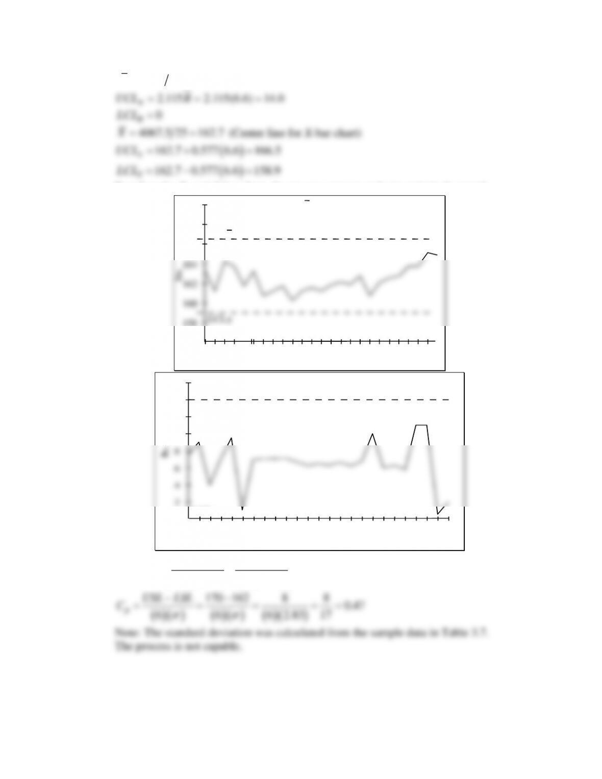
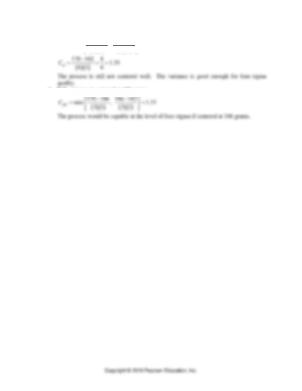
164.8 25 6.6R==
(Center line for R-chart)
0.14)6.6(115.2115.2 === RUCLR
0
R
LCL =
4067.5 25 162.7X==
(Center line for X-bar chart)
( )
162.7 0.577 6.6 166.5
x
UCL = + =
( )
162.7 0.577 6.6 158.9
x
LCL = − =
Based on the R– and X-bar chart, the process appears to be in statistical control.
170
166
160
Sample #
168
164
158
156
162
5
10
15
20
25
6
11
16
21
2
7
12
17
22
3
8
13
18
23
4
9
14
19
24
UCL
LCL
x
x
X-chart
14
10
4
Sample #
12
8
2
0
6
5
10
15
20
25
6
11
16
21
2
7
12
17
22
3
8
13
18
23
4
9
14
19
24
UCL
LCL
R
R
R-chart
16
b.
( )( ) ( )( )
170 162.7 162.7 162
min , 0.860, 0.0824 0.0824
3 2.83 3 2.83
pk
C
−−
= = =
( )( ) ( )( ) ( )( )
170 162 8 8 0.47
6 6 6 2.83 17
p
USL LSL
C
−−
= = = = =
Note: The standard deviation was calculated from the sample data in Table 3.7.
The process is not capable.
Quality and Performance ⚫ CHAPTER 3 ⚫ 3-25
c.
( )( ) ( )( )
170 163 163 162
min , 0.33
3 1 3 1
pk
C
−−
==
( )( )
170 162 8 1.33
6 1 6
p
C−
= = =
The process is still not centered well. The variance is good enough for four-sigma
quality.
d. If the process is centered at 166 grams,
( )( ) ( )( )
170 166 166 162
min , 1.33
3 1 3 1
pk
C
−−
==
The process would be capable at the level of four-sigma if centered at 166 grams.

Quality and Performance ⚫ CHAPTER 3 ⚫ 3–26
EXPERIENTIAL LEARNING: STATISTICAL PROCESS CONTROL WITH
A COIN CATAPULT *
A. Overview/Purpose
This exercise gives the students some hands-on experience in creating and using SPC
charts. Students will operate a process, collect data, develop a process control chart, and
then use the chart to monitor the process and detect any change that may occur. Maximum
efficiency is obtained by conducting this exercise after the students have read the chapter
material but before classroom lecture/discussion has taken place. Their experiences in the
exercise help give a context to the topics as they are covered in class.
B. Preparation Time Required
Instructor: Once the materials have been assembled, it should take about a half hour to
read these notes and experiment with the catapult yourself. Because the materials are
reusable, subsequent setup time should be negligible. Reproducible worksheets are
included in this teaching note (Exhibits TN.1 and TN.2). Each student should receive a
copy of each Exhibit prior to beginning the experiment.
Students: The students should read through the exercise instructions as they complete each
step.
C. Class Time Required
This exercise has been run three ways. If a 90-minute class period is available, the students
can complete both Exercise A (SPC for variables) and Exercise B (SPC for attributes). The
combined exercise can be completed in about a half hour with the remaining time for
debriefing and discussion. If time is more constrained, the teams can be divided into two
groups, one doing Exercise A and the other Exercise B. When the students have completed
the experiments, each group shares its results. This approach takes from 40 to 50 minutes.
This exercise has also been given as a homework assignment. If assigned this way, some
time should still be devoted to discussion so that the students can share their experiences
and cement their understanding of the results.
D. Conducting the Exercise
Divide the class into teams. The tasks are defined in the students’ instructions. Briefly
review the sequence of steps they will follow. Demonstrate how to catapult a coin. This
exercise needs a large, solid, flat surface; a student’s armchair will not do. Many have
chosen to work on the floor. (You may want to suggest that they dress appropriately if this
is a possibility.) Remind them about where the A2 and D3 and D4 values can be found in the
book (or, alternatively, project a table of values using an overhead projector). Then turn
them loose. The activity for each exercise will be completed in about 15 minutes.
Although separate tasks are assigned to each team member, the development of the charts
(Steps 2 and 3 in Exercise A, Step 2 in Exercise B) is best done by all team members
* This case was prepared by Dr. Larry Meile, Boston College, as a basis for classroom discussion.

Quality and Performance ⚫ CHAPTER 3 ⚫ 3-27
together. Also note that the size of the team is somewhat flexible. If you are going to have
each team do both Exercise A and B, it may be best to form three-person teams so that the
team size will be reasonable for each.
E. Debriefing/Discussion
Questions are interspersed throughout the instructions that direct the discussion. Ask the
students what they discovered. One topic will be the cause of variation in the process
(assignable cause), especially for catapulting the coins into the cup. Some students will
come up with methods for releasing the catapult (other than with their finger) that will
greatly reduce process variability. Take advantage of this to bring into the discussion the
concept of robust process design. Ask them how many samples need to be taken to detect a
change (if a change is present). This will lead into an analysis of the data patterns that
reveal a change in the process, even if a point is not outside one of the control limits.
Bring up the topic of monitoring the process as it occurs, rather than after the fact. Point
out how control would be lost if the data were collected throughout the day and analyzed
only at the end.
You may want to discuss the concept of sampling the output. This exercise is somewhat
artificial because units of output were not produced, from which a random sample was
drawn.
In Exercise B, you may find a wide range of abilities exhibited when students try to flip the
coin into a cup. Some students will be able to land the coin in the cup so consistently that
no errors show up in the 10-trial samples. Others will struggle to get it in even half the
time. Use this variation to drive a discussion of when it is appropriate to use SPC and what
the percent of defects has on the chart’s control limits. This also leads well into a
discussion of sample size. In Exercise B, for example, the sample size may have to be
increased to find, on the average, at least two defects per sample.
Another concept to explore with this experiment is a confidence interval and the effect of
altering the number of standard deviations used to establish the UCL and LCL.
Many other topics can arise from these exercises as well. The more times you run this
exercise in class, the more topics you will find to explore. This exercise can also be easily
extended to show the use of the standard deviation method for determining control limits
for variable sampling.
Quality and Performance ⚫ CHAPTER 3 ⚫ 3–28
EXHIBIT TN.1
Coin Catapult Worksheet
EXERCISE A
Data Table
Sample
Observation
Sample
Sample
Number
1
2
3
4
5
Mean
x
Range R
1
2
3
4
x=
R=
2
4
6
8
Sample
1
3
5
7
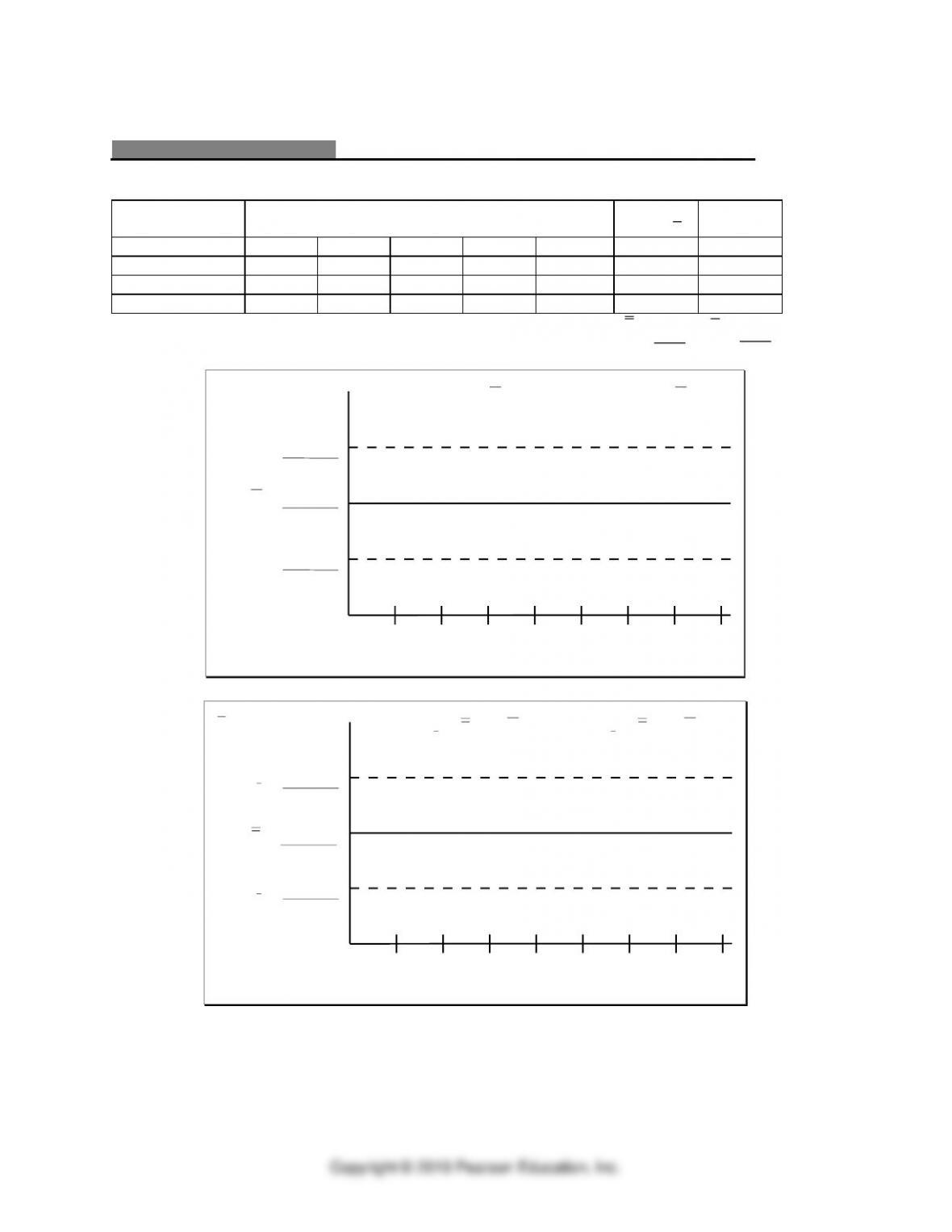
R-chart
UCL
R
=
LCL
R
=
R
=
UCL
D
R
R
=
4
LCL
D
R
R
=
3
2 4 6 8
Sample
1 3 5 7
-chart
xUCL x A R
x= + 2LCL x A R
x= − 2
UCLx=
LCLx=
x=
Quality and Performance ⚫ CHAPTER 3 ⚫ 3-29
EXHIBIT TN.1 (Cont.)
Coin Catapult Worksheet
Data Table (for additional observations)
Sample
Sample
Sample
Observation
Mean
Range
Number
1
2
3
4
5
x
R
5
6
7
8
EXHIBIT TN.2
Exercise B
Data Table
Sample
Observation
Number
1
2
3
4
5
6
7
8
9
10
Misses
p
1
2
3
4
pn
=misses
First, calculate the average fraction defective,
p
.
p=total defects
total observations
p=
Next, calculate the standard deviation of the distribution of
p
. Remember that n represents
the sample size (in this case 10), not the number of samples or the total number of
observations.
p
p p
n
=−
( )
1
p=
Now determine the confidence level for the UCL and LCL. This is the number of standard
deviations required for a two-tailed confidence interval. Frequently a 3-sigma value is used
to obtain a 99% confidence interval, although other intervals can be used as well. For this
example use 3 sigmas (z = 3).
Finally, using the values determined above, develop the UCL and LCL.
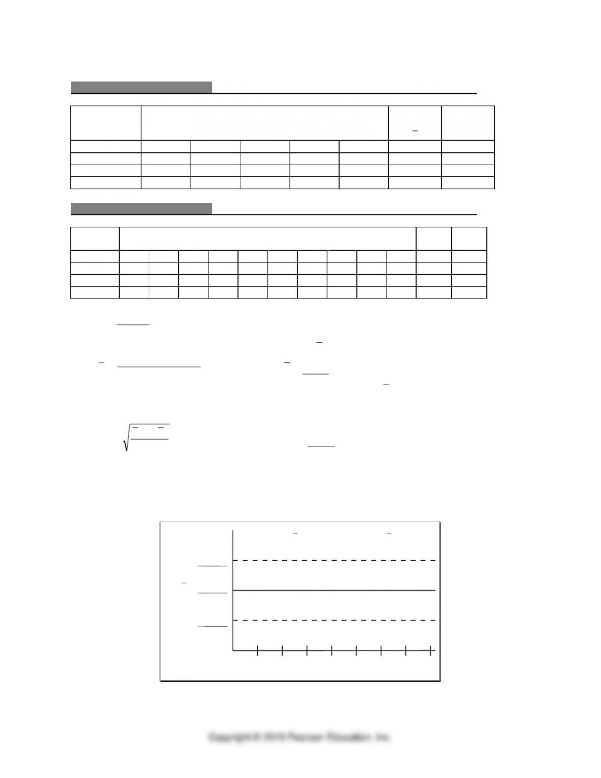
2
4
6
8
Sample
1
3
5
7
-chart
UCL
p
=
LCL
p
=
p
=
p
UCL
p
z
p
p
=
+
LCL
p
z
p
p
=
−