
219
Chapter 8
Risk and Return
LEARNING OBJECTIVES (Slides 8-2 & 8-3)
1. Calculate profits and returns on an investment and convert holding period returns to annual
returns.
2. Define risk and explain how uncertainty relates to risk.
3. Appreciate the historical returns of various investment choices.
4. Calculate standard deviations and variances with historical data.
5. Calculate expected returns and variances with conditional returns and probabilities.
6. Interpret the trade-off between risk and return.
7. Understand when and why diversification works at minimizing risk and understand the
difference between systematic and unsystematic risk.
8. Explain beta as a measure of risk in a well-diversified portfolio.
9. Illustrate how the security market line and the capital asset pricing model represent the
two-parameter world of risk and return.
IN A NUTSHELL…
In this chapter, the author discusses various topics related to the risk and return of financial
assets. The measurement of holding period return and its conversion into annualized rates of
return on investments is covered first, followed by the definition of risk. After providing a bit of
perspective on the nature of historical returns characterizing securities markets, the author
explains how standard deviation and variance can be used to measure historical or ex-post risk.
Next, the calculation of expected or ex-ante risk and return measures is illustrated using a
probability distribution framework, along with a discussion of the trade-off between risk and
LECTURE OUTLINE
8.1 Returns (Slides 8-4 to 8-13)
In order to analyze the performance of an investment it is important that investors learn how to
measure returns over time. Furthermore, because return and risk are intricately related, the
measurement of return also helps in the understanding of the riskiness of an investment.
Dollar Profits and Percentage Returns: Investment performance can be measured in terms
of the profit or loss derived from holding it for a period of time. Some investments, such as

220 Brooks ◼ Financial Management: Core Concepts, 4e
stocks and bonds, provide periodic income in the form of dividends or interest, in addition to
capital gains (or losses) arising from price changes. Thus, a generic formula for measuring the
dollar profit (or loss) on an investment is as follows:
Dollar Profit or Loss = Ending value + Distributions – Original Cost (8.1)
Dollar profits being absolute values do not provide a good gauge of the relative performance of
an investment. In other words, is a $2 profit on a $10 investment just as good as a $2 profit on a
$100 investment? Obviously not! Hence we calculate the rate of return or percentage return on
an investment as follows:
Dollar Profit or Loss
Rate of return Original Cost
=
Also, since investments can be held for varying periods of time before being disposed off or
closed out, an alternative name for overall performance of an investment is holding period
return (HPR) and is measured in any one of the three following methods:
Profit
Cost
HPR =
(8.3a)
Ending price Distributions Beginning price
Beginning price
Example 1: Calculating dollar and percentage returns
Joe bought some gold coins for $1,000 and sold those four months later for $1,200. Jane on the
other hand bought 100 shares of a stock for $10 and sold those two years later for $12 per share
after receiving $0.50 per share as dividends for the year. Calculate the dollar profit and
percentage return earned by each investor over their respective holding periods.
Joe’s Dollar Profit = Ending value – Original cost
Chapter 8 ◼ Risk and Return 221
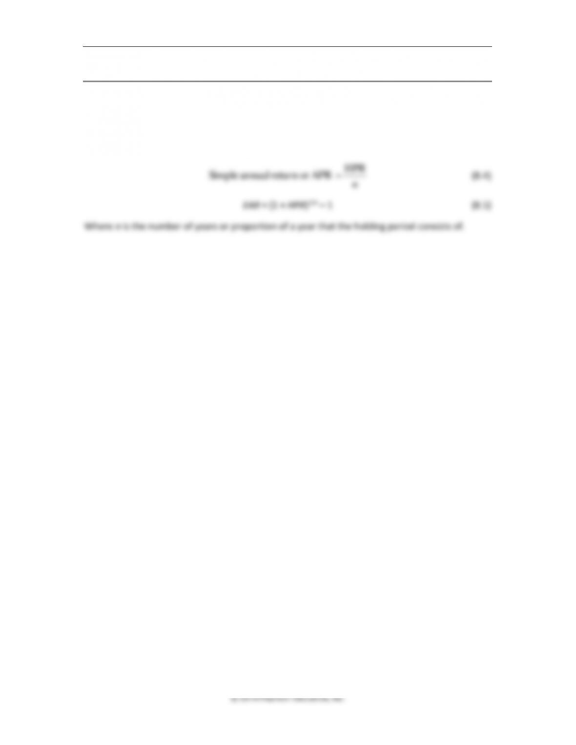
Converting Holding Period Returns to Annual Returns: For meaningful comparisons of
investment performance, in cases of varying holding periods, it is essential to state HPRs in
terms of either simple (annual percentage rate, APR) or compound annual returns (effective
annual rate, EAR) by using the following conversion formulas:
HPR

222 Brooks ◼ Financial Management: Core Concepts, 4e
Example 2: Comparing HPRs
Given Joe’s HPR of 20% over four months and Jane’s HPR of 25% over two years, is it correct to
conclude that Jane’s investment performance was better than that of Joe?
ANSWER: Compute each investor’s APR and EAR and then make the comparison.
Extrapolating Holding Period Returns: It is important to remind students that although the
extrapolation of short-term HPRs into APRs and EARs is mathematically correct, it often tends to
be highly unrealistic and practically impossible to achieve, especially with very short holding
periods.
Extrapolation implies earning the same periodic rate over and over again throughout the
relevant number of times per year.
Hence, if the holding period is fairly short, and the HPR fairly high, extrapolation would lead to
huge numbers, as shown in Example 3 below.
Example 3: Unrealistic nature of APR and EAR
Let’s say you buy a share of stock for $2 and sell it a week later for $2.50. Calculate your HPR,
APR, and EAR. How realistic are the numbers?


Chapter 8 ◼ Risk and Return 225
1993
9.87%
–9.12%
0.0083174
1994
1.29%
–17.70%
0.031329
1995
37.71%
18.72%
0.0350438
1996
23.07%
4.08%
0.0016646
1997
33.17%
14.18%
0.0201072
1998
28.58%
9.59%
0.0091968
1999
21.04%
2.05%
0.0004203
Total
189.90%
0.18166156
Average
18.99%
Variance
0.020184618
Stand. Dev
14.207%
( )
2
R Mean 0.18166156
Variance 0.020184618
N 1 10 1
−
= = =
−−
Standard Deviation = √Variance = √.020184618 = 14.207%
Normal Distributions:
Figure 8.2 is a standard normal bell-shaped curve with a mean of zero and a standard deviation
of one. If data are normally distributed, it lets the researcher or analyst make the following
inferences regarding the expected values of the data:
1. About 68% of all observations of the data fall within one standard deviation of the average:
the mean plus one or minus one standard deviation (add the 34% on the right of the mean
with a corresponding 34% on the left of the mean).
2. About 95% of all observations of the data fall within two standard deviations of the mean:
the mean plus two or minus two standard deviations.

Chapter 8 ◼ Risk and Return 227
concluded that the higher the return one expects the greater would be the risk (variability of
return) that one would have to tolerate.
8.5 Returns in an Uncertain World
(Expectations and Probabilities) (Slides 8-25 to 8-28)
When we are contemplating making an investment, it is the expected or ex-ante returns and risk
measures that are more relevant than the ex-post measures that we have covered so far.
To calculate ex-ante measures the various scenarios with their possible outcomes and
probabilities are estimated, listed in a probability distribution, and then the expected return and
risk measures are estimated using Equations 8.8 and 8.9 (as shown below):
expected payoff = payoff probabilityi
i
8.8
22
(payoff expected payoff ) probability
ii
= −
8.9
Determining the Probabilities of All Potential Outcomes. When setting up probability
distributions, the following two rules must be followed:
1. The sum of the probabilities must always add up to 1.0 or 100%.
2. Each individual probability estimate must be positive. We cannot have a negative probability
value.
Example 5: Expected return and risk measurement
Using the probability distribution shown below, calculate Stock XYZs expected return, E(r), and
standard deviation σ (r).
State of the
Economy
Probability of
Economic State
Return in
Economic State
Recession
45%
–10%
Steady
35%
12%
Boom
20%
20%

Chapter 8 ◼ Risk and Return 229
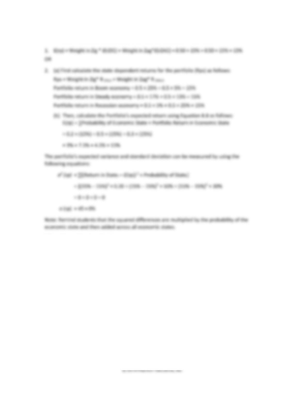
The Portfolio’s expected return, E(rp), return can be measured in two ways.
When Diversification Works:
The benefits of diversification are best realized by combining stocks that are not perfectly
positively correlated with each other.
The more negatively correlated a stock is with the other stocks in an investment portfolio, the
greater will be the reduction in risk achieved by adding it to the portfolio.
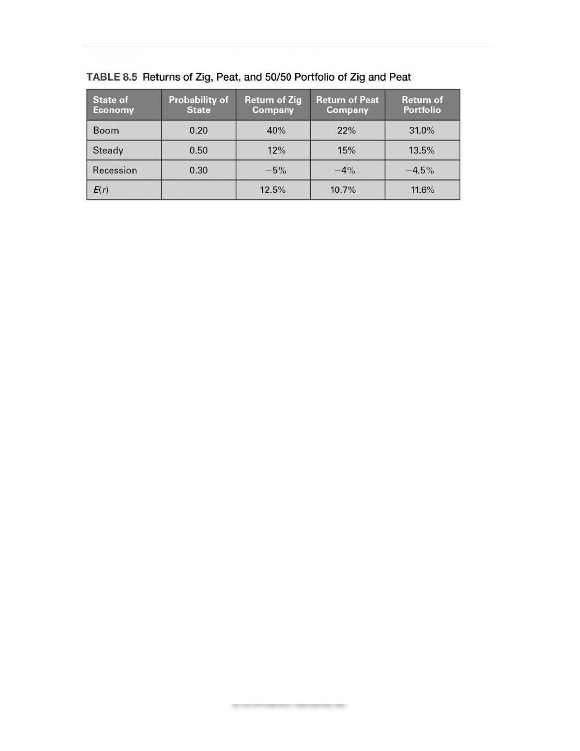
Table 8.5 presents a probability distribution of returns for two stocks, The Zig Co., and The Peat
Co., and for an equally weighted portfolio of the two stocks as well.
230 Brooks ◼ Financial Management: Core Concepts, 4e

Chapter 8 ◼ Risk and Return 231
Using the data from Table 8.5 we get the following risk-return measures
Zig
Peat
50-50 Portfolio
E(r)
12.5%
10.70%
11.60%
Std. Dev.
15.6%
10.00%
12.44%
Figure 8.10 plots the risk-return profiles of the three investments and illustrates the
diversification benefit derived from combining these two stocks into a portfolio.
The portfolio has an expected return that is equivalent to the weighted average returns of the
two stocks, but its standard deviation or risk (12.44%) is lower than the weighted average of the
two standard deviations (12.8%).
The portfolio’s risk-return combination plots above the line joining the risk-return combinations
of the two stocks, indicating that the portfolio’s expected return is higher than what would have
been expected based on the weighted average risk of the two stocks.
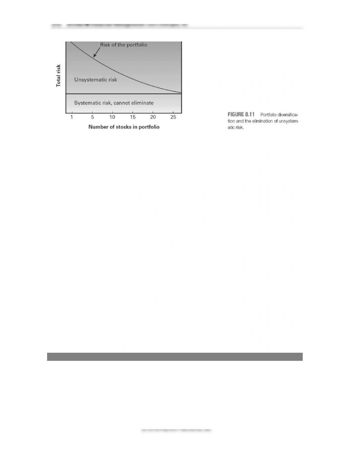
Adding More Stocks to the Portfolio: Systematic and Unsystematic Risk
The total risk of an investment can be broken down into two parts: unsystematic or diversifiable
risk and systematic or nondiversifiable risk.
Unsystematic risk or company-specific risk can be diversified away by efficient portfolio

Chapter 8 ◼ Risk and Return 233
Y $30,000 0.2000 1.3
Z $45,000 0.3000 0.8
We have introduced two different measures of risk related to financial assets; standard
deviation (or variance) and beta.
The standard deviation is a measure of the total risk of an asset, both its systematic and
unsystematic risk.
Beta is a measure of an asset’s systematic risk. When we view any one of our assets as part of a
well-diversified portfolio, it is proper to use beta as the measure of risk for the asset.
If we do not have a well-diversified portfolio, it is more prudent to use standard deviation as the
measure of risk for our asset.
8.9 The Capital Asset Pricing
Model and the Security Market Line (Slides 8-49 to 8-61)
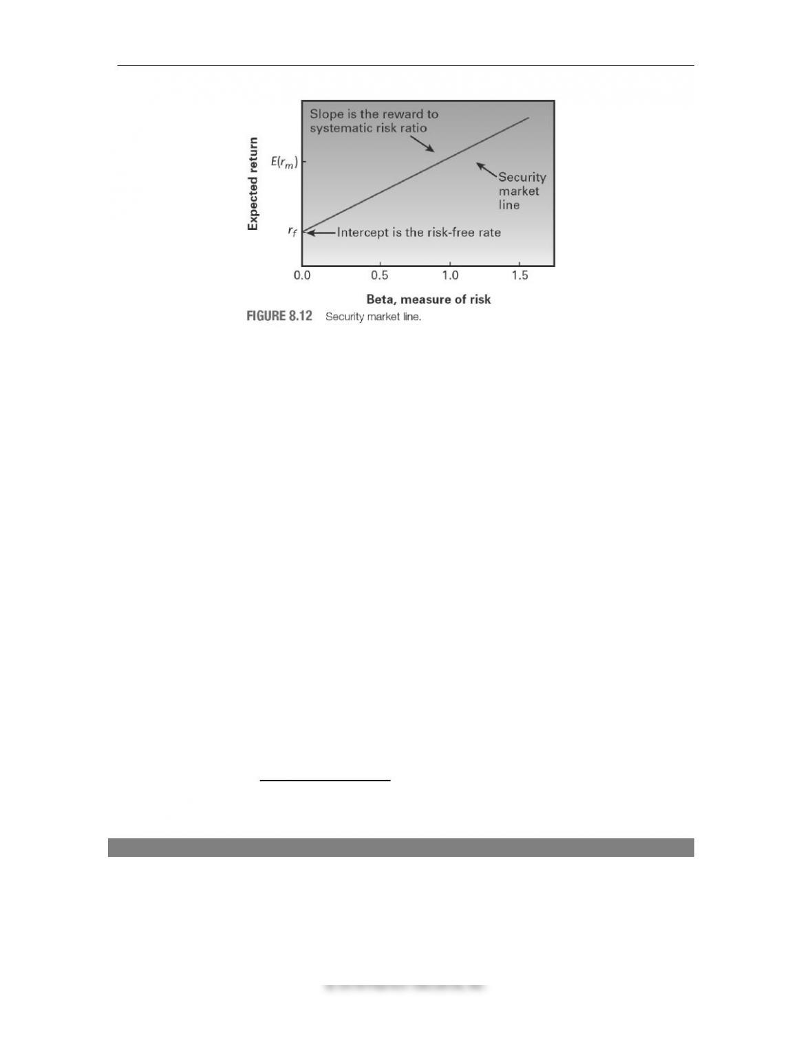
The security market line (SML), shown below in Figure 8.12, is a graphical depiction of the
relationship between an asset’s required rate of return and its systematic risk measure, i.e. beta.
It is based on three assumptions.
Assumption 1: There is a basic reward for waiting: the risk-free rate. This means that an investor
could earn the risk-free rate by delaying consumption.
These three assumptions imply that the SML is upward sloping, has a constant slope (linear),
and has the risk-free rate as its y-intercept.
234 Brooks ◼ Financial Management: Core Concepts, 4e
The Capital Asset Pricing Model (CAPM) is the equation form of the SML and is used to
quantify the relationship between the expected rate of return and the systematic risk of
individual securities as well as portfolios.
It states that the expected return of an investment is a function of
1. The time value of money (the reward for waiting)
2. A reward for taking on risk
3. The amount of risk
The equation representing the CAPM (Equation 8.11 as shown below) is in effect a straight line
equation of the form:
y a b x= +
Where, y is the value of the function, a is the intercept of the function, b is the slope of the line,
and × is the value of the random variable on the x-axis.
By substituting expected return E(ri) for the y variable, the risk-free rate rf for the intercept a,
the market risk premium, (E(rm) – rf) for the slope b, and the systematic risk measure, β, for the
random variable on the x-axis, we have the formal equation for the SML.
( ) [ ( ) ]
i f m f i
E r r E r r
= + − 8.11
Note: Students often assume that beta is the slope of the SML. Emphasize the point that the
slope of the SML is the market risk premium, i.e., (E(rm) – rf), and not beta, which is on the x-
axis. If investors demand a higher risk premium to bear average risk, the slope of the SML will
increase and vice versa.
Example 7: Finding expected returns for a company with known beta
The New Ideas Corporation’s recent strategic moves have resulted in its beta going from 0.8 to
1.2. If the risk-free rate is currently at 4% and the market risk premium is being estimated at 7%,
calculate its expected rate of return.
Using the CAPM equation we have:

Chapter 8 ◼ Risk and Return 235
© 2016 Pearson Education, Inc.
( ) [ ( ) ]
i f m f i
E r r E r r
= + − 8.11
Where;
Rf = 4%; E(rm) – rf = 7%; and β = 1.2
Expected rate of return = 4% + 7% × 1.2 = 4% + 8.4 = 12.4%
Note: Students often forget their rules of operation. Remind them to first multiply 7% × 1.2 =
8.4; and then add 4% = 12.4%.
Application of the SML
Although the SML was primarily developed as a way of explaining the relationship between an
asset’s expected return and risk, it has many practical applications, including the following:
1. To determine the prevailing market or average risk premium, given the expected returns of
a couple of stocks and their betas
Example 8: Determining the market risk premium
Stocks X and Y seem to be selling at their equilibrium values as per the opinions of the majority
of analysts. If Stock X has a beta of 1.5 and an expected return of 14.5%, and Stock Y has a beta
of 0.8 and an expected return of 9.6%, calculate the prevailing market risk premium and the risk–
free rate.
Because the market risk premium is the slope of the SML, i.e., [E(rm) – rf], we can solve for it as
follows:


Chapter 8 ◼ Risk and Return 237
Questions
1. What are the two parameters for selecting investments in the finance world? How do
investors try to get the most out of their investment with regard to these two
parameters?
2. What are the two ways to measure performance in the finance world?