76
Chapter 4
The Time Value of Money (Part 2)
LEARNING OBJECTIVES (Slides 4-2 to 4-3)
1. Compute the future value of multiple cash flows.
2. Determine the future value of an annuity.
3. Determine the present value of an annuity.
4. Adjust the annuity formula for present value and future value for an annuity due and
understand the concept of a perpetuity.
5. Distinguish among the different types of loan repayments: discount loans, interest-only
loans, and amortized loans.
6. Build and analyze amortization schedules.
7. Calculate waiting time and interest rates for an annuity.
8. Apply the time value of money concepts to evaluate the lottery cash flow choice.
9. Summarize the ten essential points about the time value of money.
IN A NUTSHELL…
In part two of this two-part unit on the time value of money topic, the author discusses and
illustrates how the time value of money equation can be modified and used for calculations
involving the compounding and discounting of interest in cash flow streams that are more
complex that mere lump sums. Real life situations seldom involve single outflow/inflow
LECTURE OUTLINE
4.1 Future Value of Multiple Payment Streams (Slides 4-4 to 4-8)
In the case of investments involving unequal periodic cash flows, we can calculate the
future value of the cash flows by treating each of the cash flows as a lump sum and
calculate its future value over the relevant number of periods. The individual future values
are then summed up to get the future value of the multiple payment streams.
Chapter 4 ◼ The Time Value of Money (Part 2) 77
It is best to use a time line, as shown in Figure 4-1 in the text, which clearly shows each
cash flow, the respective number of periods over which interest is to be compounded, and
the interest rate that will apply.
There is a shorter alternative way to solve the future value of a stream of unequal periodic
cash flows, which involves using the Net Present Value (NPV) function of a financial
calculator or a spreadsheet. We can first compute the net present value (at t = 0) of the
stream of uneven cash flows at the given rate of interest, and then using the NPV as the
present value, we find the future value of a lump sum at the end point of the cash flow
stream. This method is shown in Example 1 below.
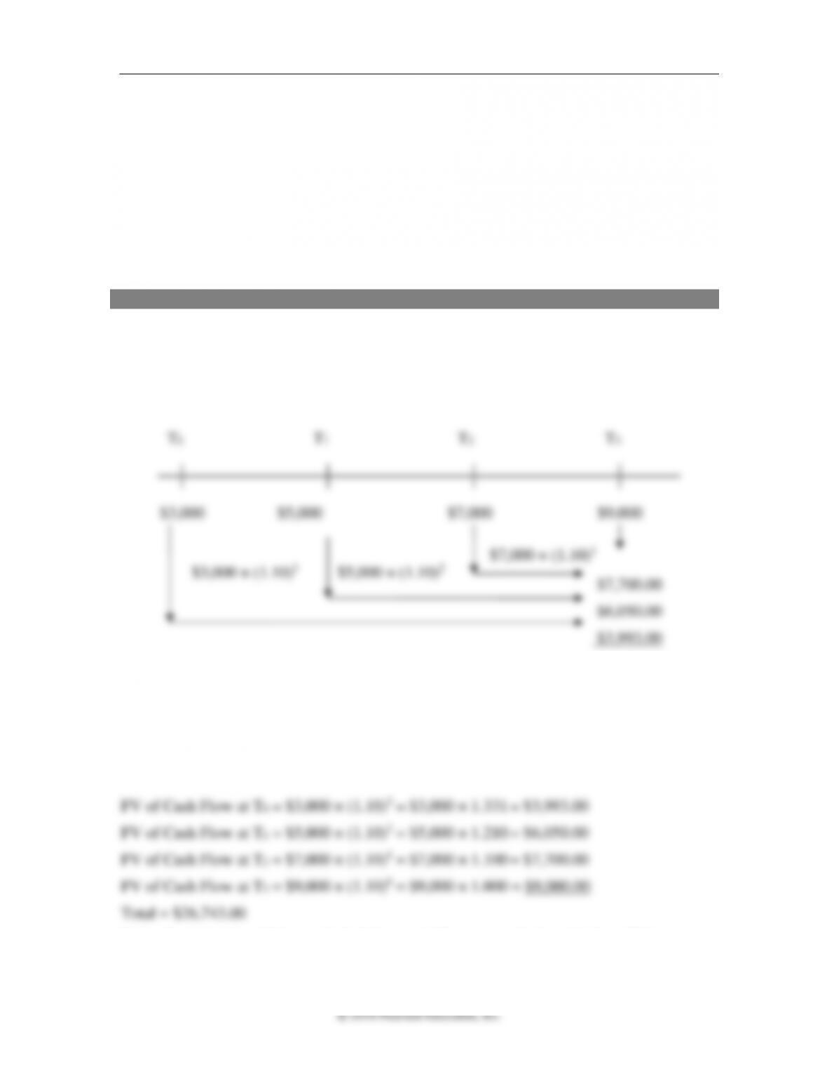
Example 1: Future value of an uneven cash flow stream
Jim deposits $3,000 today into an account that pays 10% per year, and follows it up with
three more deposits at the end of each of the next three years. Each subsequent deposit is
$2,000 higher than the previous one. How much money will Jim have accumulated in his
account by the end of three years?
We use the Future Value of a Single Sum formula and compound each cash flow for the
relevant number of years over which interest will be earned. Then we sum up the
compounded values to get the accumulated value of Jim’s deposits at the end of three years
as shown below:
FV = PV × (1 + r)n
Note: Students should be reminded that cash flows can only be added up if they occur
at the same point in time as at the end of Year 3.
$3,000 $5,000 $7,000 $9,000
T0 T1 T2 T3
$7,700.00
$6,050.00
$3,993.00
$3,000 × (1.10)3
$5,000 × (1.10)2
$7,000 × (1.10)1

© 2018 Pearson Education, Inc.
4.2 Future Value of an Annuity Stream (Slides 4-9 to 4-14)
Often, we are faced with financial situations which involve equal, periodic outflows and
inflows. Such payment streams are known as annuities. Examples of an annuity stream
include rent, lease, mortgage, car loan, and retirement annuity payments. An annuity stream
can begin at the start of each period as is true of rent and insurance payments or at the end
of each period, as in the case of mortgage and loan payments. The former type is called an
annuity due, while the latter is known as an ordinary annuity stream. This section covers
ordinary annuities. Annuities due will be covered in a later section.
Although the future value of an ordinary annuity stream can be calculated by using the
same process that was explained in section 4.1, there is a simplified formula that makes the
process much easier. The formula for calculating the future value of an annuity stream is as
follows:
( )
+−
=
11
n
r
FV PMT r
where PMT is the term used for the equal periodic cash flow, r is the rate of interest, and n
is the number of periods involved. The item that PMT is multiplied by is known as the
Future Value Interest Factor of an Annuity (FVIFA). It can be either calculated using the
equation or got from a table provided in Appendix A-3. Of course, table values are only
available for discrete interest rates and time periods.
Note: The length of the period can be a day, week, quarter, month, or any other equal
unit of time, not just a year as is often misunderstood by students. The rate of interest,
however, is often given on an annual basis and must be accordingly adjusted and used
in the problem.
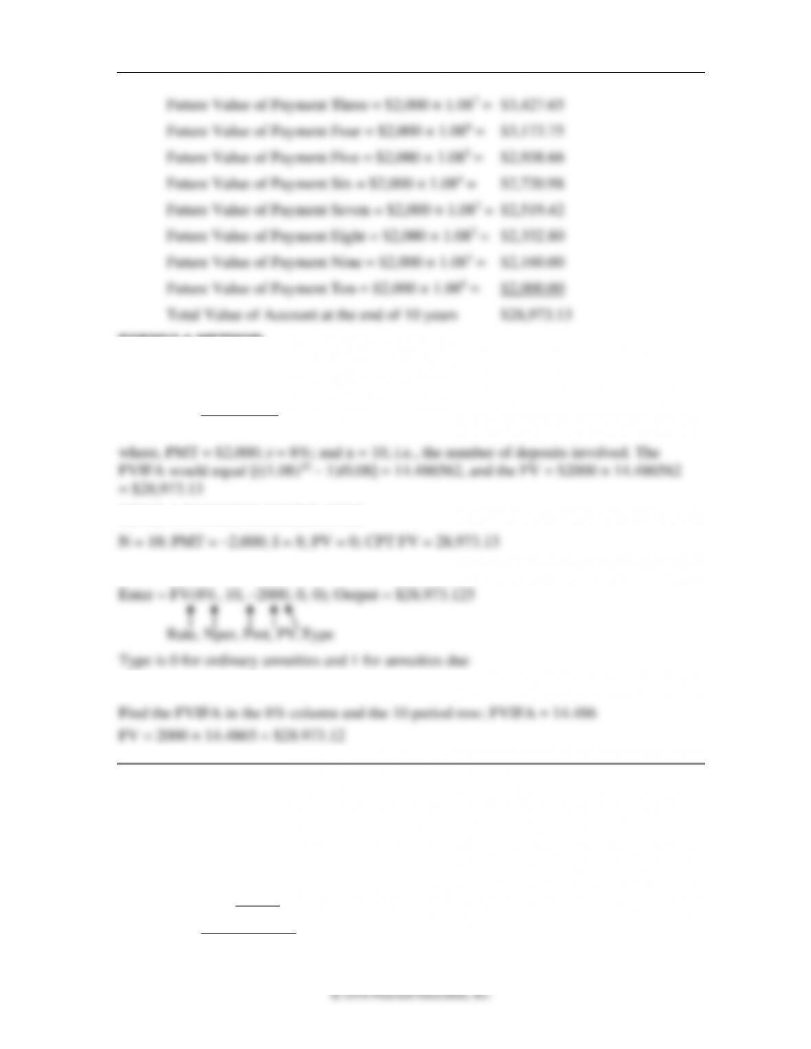
Example 2: Future value of an ordinary annuity stream
Jill has been faithfully depositing $2,000 at the end of each year for the past ten years into
an account that pays 8% per year. How much money will she have accumulated in the
account?
Chapter 4 ◼ The Time Value of Money (Part 2) 79
© 2018 Pearson Education, Inc.
Future Value of Payment Three = $2,000 × 1.087 = $3,427.65
Future Value of Payment Four = $2,000 × 1.086 = $3,173.75
Future Value of Payment Five = $2,000 × 1.085 = $2,938.66
Future Value of Payment Six = $2,000 × 1.084 = $2,720.98
Future Value of Payment Seven = $2,000 × 1.083 = $2,519.42
Future Value of Payment Eight = $2,000 × 1.082 = $2,332.80
Future Value of Payment Nine = $2,000 × 1.081 = $2,160.00
Future Value of Payment Ten = $2,000 × 1.080 = $2,000.00
Total Value of Account at the end of 10 years $28,973.13
FORMULA METHOD
It is much quicker to solve this problem using the following formula:
( )
+−
=
11
n
r
FV PMT r
USING A FINANCIAL CALCULATOR
USING AN EXCEL SPREADSHEET
USING FVIFA TABLE A-3
4.3 Present Value of an Annuity (Slides 4-15 to 4-20)
If we are interested in finding the value of a series of equal periodic cash flows at the
current point in time, we can either sum up the discounted values of each periodic cash
flow (PMT) for the related number of periods or use the following simplified formula:
( )
−
+
=
1
11n
r
PV PMT r
80 Brooks ◼ Financial Management: Core Concepts, 4e
The last portion of the equation,
( )
−
+
1
11n
r
r
, is the Present Value Interest Factor of
an Annuity (PVIFA). The values of various PVIFAs are displayed in Appendix A-4 for
different combinations of discrete interest or discount rates (r) and the number of payments
(n). A practical application of such a calculation would be in calculating how much to have
saved up in an account prior to a child attending college or prior to retirement so as to be
able to withdraw equal annual amounts each year over a required number of years.
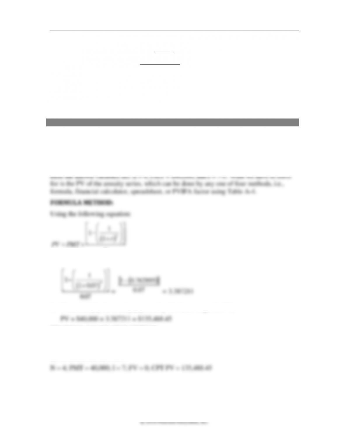
Example 3: Present value of an annuity
John wants to make sure that he has saved up enough money prior to the year in which his
daughter begins college. Based on current estimates, he figures that college expenses will
amount to $40,000 per year for four years (ignoring any inflation or tuition increases during
the four years of college). How much money will John need to have accumulated in an
account that earns 7% per year, just prior to the year that his daughter starts college?
1. Calculate the PVIFA value for n = 4 and r = 7%.
( )
−
+
4
1
11 0.07
0.07
2. Then, multiply the annuity payment by this factor to get the PV,
FINANCIAL CALCULATOR METHOD:
It is important to remind students that the calculator must be in END mode so that the
payments are treated as an ordinary annuity. Set the calculator for an ordinary annuity
(END mode) and then enter:
( )
07.0
762895.01−
© 2018 Pearson Education, Inc.
4.4 Annuity Due and Perpetuity (Slides 4-21 to 4-26)
Annuity due
Certain types of financial transactions such as rent, lease, and insurance payments involve
equal periodic cash flows that begin right away or at the beginning of each time interval.
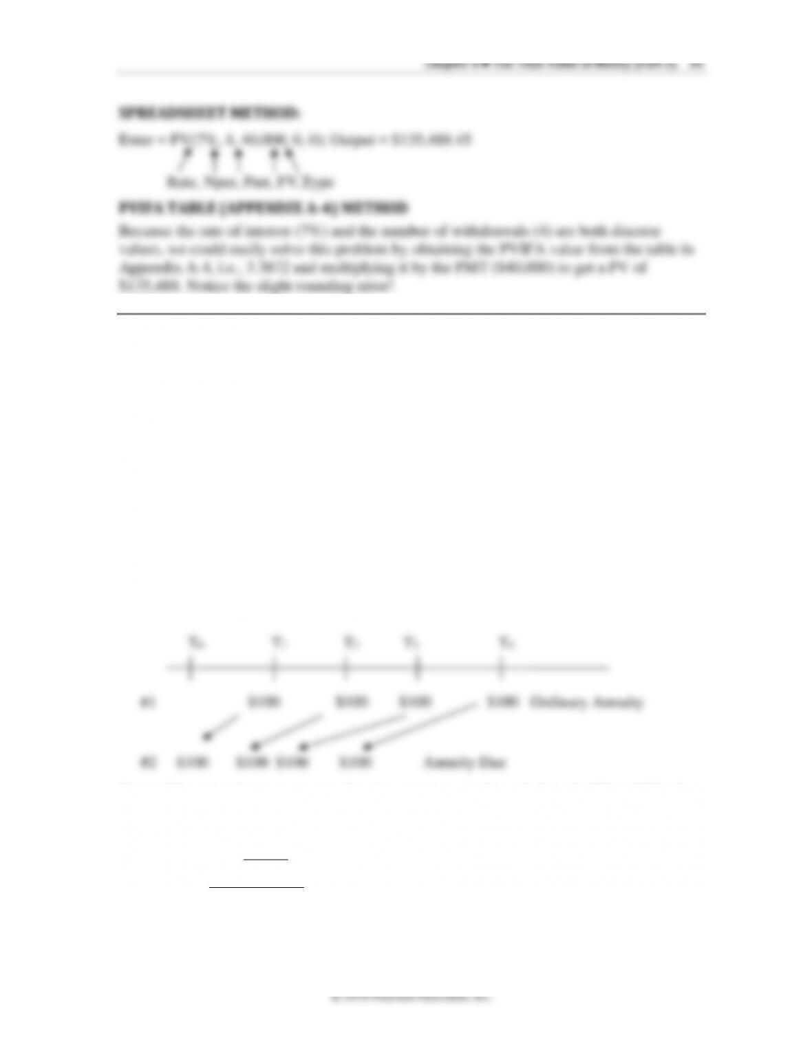
This type of annuity is known as an annuity due. Figure 4.5 in the text shows both types of
annuities on a time line. An annuity due stream is scaled back for one period as shown by
the arrows. Note that when calculating the PV of an annuity due stream one less period of
interest would be required for each payment because the first cash flow begins right away.
Likewise, when calculating the FV of the cash flow stream at the end of four periods, an
additional period of interest would apply to each periodic cash flow, since the fourth
payment occurs at the beginning of the fourth year.
Figure 4.5
Ordinary Annuity versus Annuity Due
For problems involving an annuity due, the equations used to calculate the PV and FV of an
ordinary annuity can simply be adjusted by multiplying them by the term (1 + r). That is,
( ) ( )
−
+
= +
1
111
n
r
PV PMT r
r
T0
#1
$100 $100 $100 $100 Ordinary Annuity
T1
T2
T3
T4
#2
$100 $100 $100 $100 Annuity Due
82 Brooks ◼ Financial Management: Core Concepts, 4e
Or
PV annuity due = PV ordinary annuity × (1 + r)
AND
( ) ( )
+−
= +
11
1
n
r
FV PMT r
r
4.6
Or
FV annuity due = FV ordinary annuity × (1 + r)
When using a financial calculator we must set the mode to BGN for an annuity due or END
for an ordinary annuity and proceed just as we would any other PV or FV problem.
In the case of a spreadsheet, the “Type” of the cash flow, within the = PV or = FV
functions is set to “0” or omitted for an ordinary annuity and “1” for an annuity due.
Example 4: Annuity due versus ordinary annuity
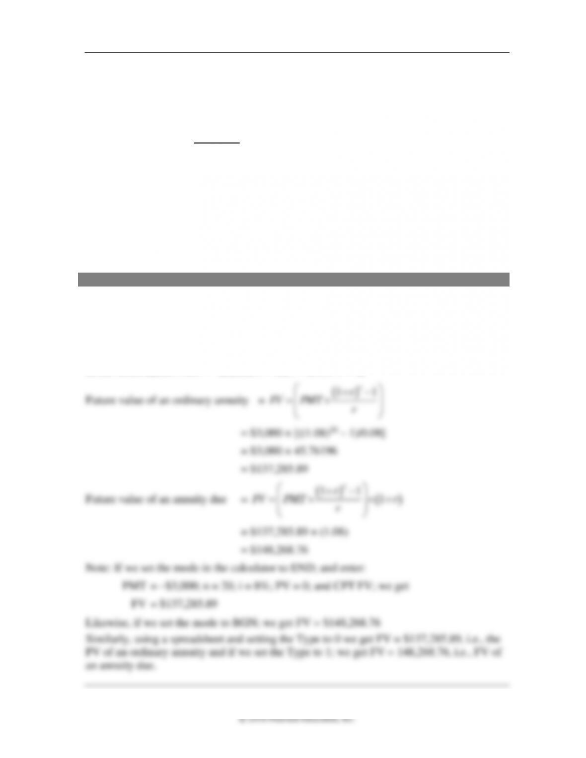
Let’s say that you are saving up for retirement and decide to deposit $3,000 each year for
the next twenty years into an account which pays a rate of interest of 8% per year. By how
much will your accumulated nest egg vary if you make each of the twenty deposits at the
beginning of the year, starting right away, rather than at the end of each of the next twenty
years?
Given information: PMT = –$3,000; n = 20; i = 8%; PV = 0;
( )
+−
11
n
r
Chapter 4 ◼ The Time Value of Money (Part 2) 83
Perpetuity
A perpetuity is an equal periodic cash flow stream that will never cease. One example of
such a stream is a British consol, which is a bond issued by the British government that
promised to pay a specified rate of interest forever, without ever repaying the principal.
The PV of a perpetuity is calculated by using the following equation:
Example 5: PV of a perpetuity
If you are considering the purchase of a consol that pays $60 per year forever, and the rate
of interest you want to earn is 10% per year, how much money should you pay for the
consol?
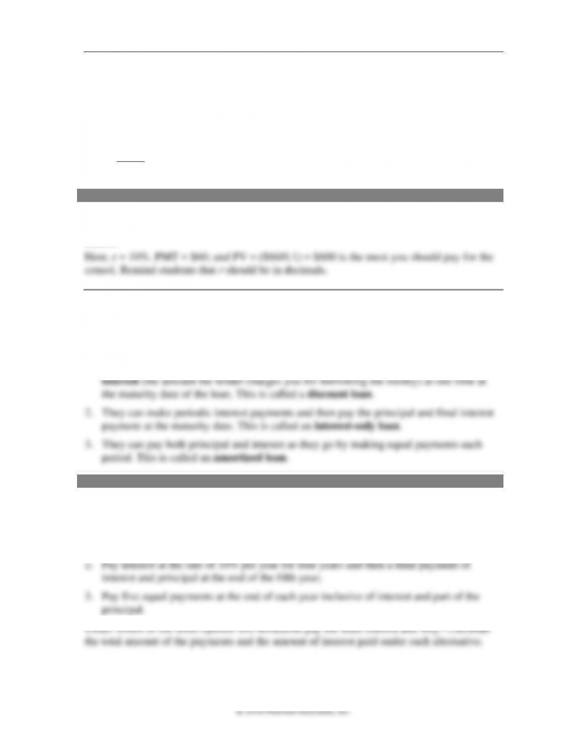
4.5 Three Loan Payment Methods (Slides 4-27 to 4-32)
Depending on the terms agreed upon at the time of issue, borrowers can typically pay off a
loan in one of three ways:
1. They can pay off the principal (the original loan amount that you borrowed) and all the
Example 6: Discount versus interest-only versus amortized loans
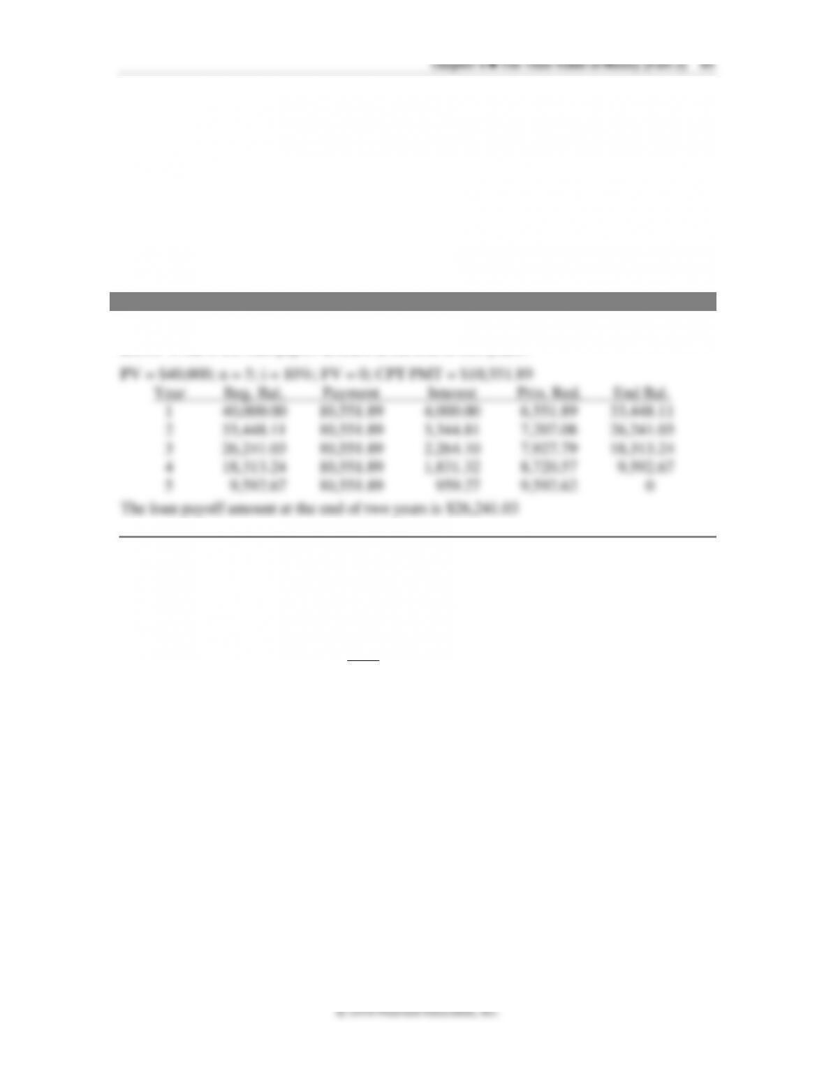
Roseanne wants to borrow $40,000 for a period of five years. The lender offers her a
choice of three payment structures:
1. Pay all of the interest (10% per year) and principal in one lump sum at the end of five
years;
r
PMT
PV =
84 Brooks ◼ Financial Management: Core Concepts, 4e
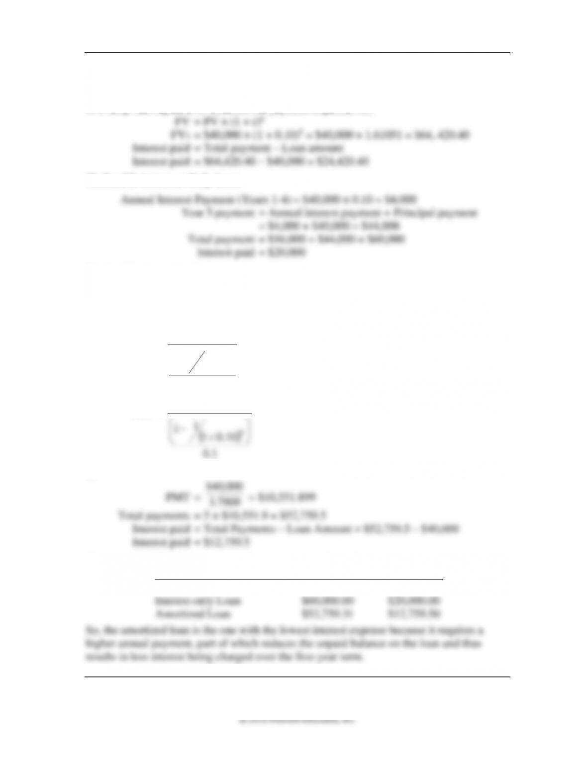
Method 1: Discount Loan
Because all the interest and the principal are paid at the end of five years we can use the FV
of a lump sum equation to calculate the payment required, i.e.,
Method 2: Interest-Only Loan
Method 3: Amortized Loan
To calculate the annual payment of principal an interest we can use the PV of an ordinary
annuity equation and solve for the PMT value using n = 5, I = 10%, PV = $40,000, and
FV = 0. That is:
4.9
or
Comparison of Total payments and interest paid under each method
Loan Type Total Payment Interest Paid
Discount Loan $64,420.40 $24,420.40
( )
r
r
PV
PMT
n
+
−
=
1
1
1
( )
1.0
10.01
1
1
000,40$
5
+
−
=PMT
000,40$
86 Brooks ◼ Financial Management: Core Concepts, 4e
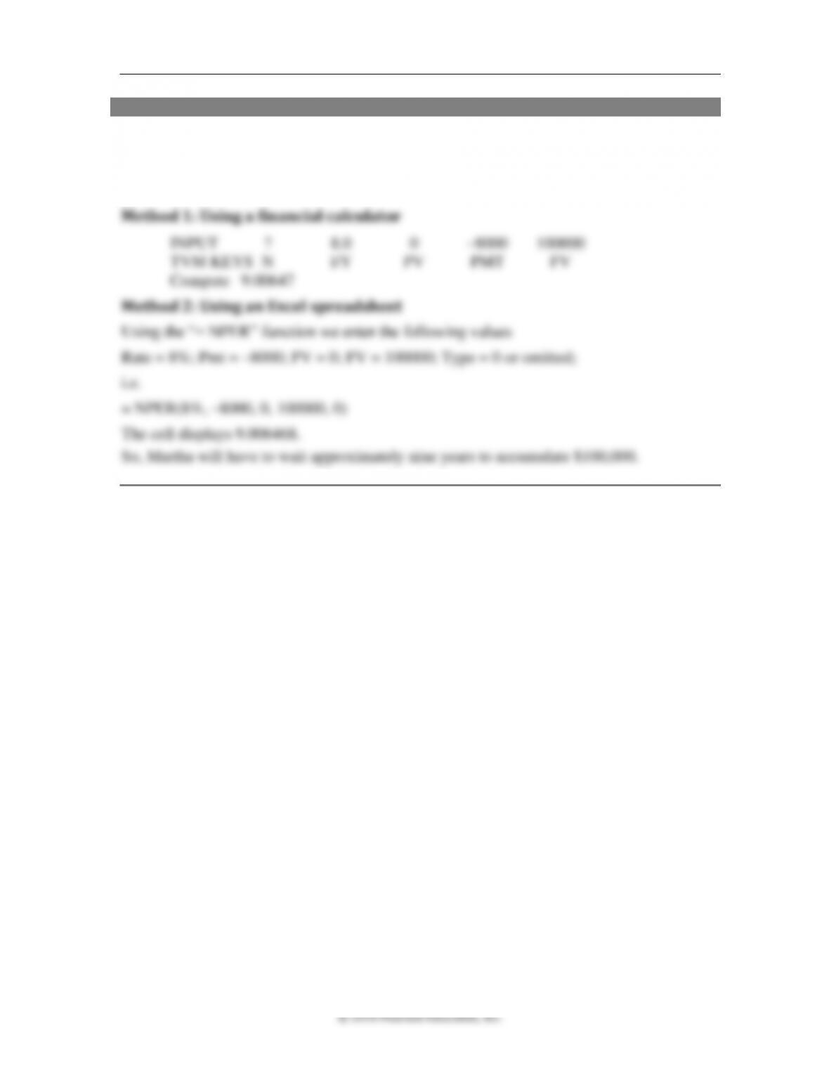
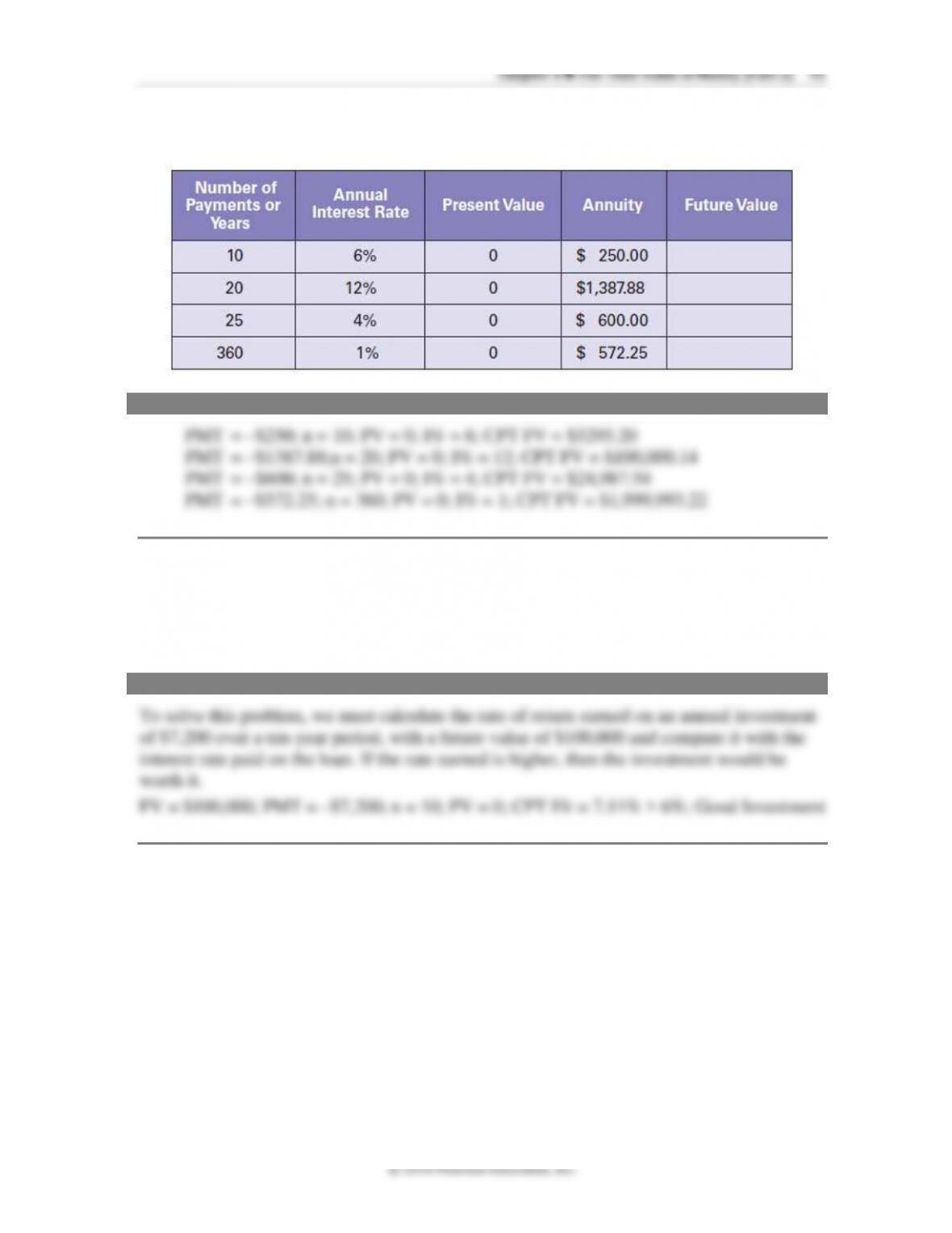
Example 8: Solving for the number of annuities involved
Martha wants to save up $100,000 as soon as possible so that she can use it as a down
payment on her dream house. She figures that she can easily set aside $8,000 per year and
earn 8% annually on her deposits. How many years will Martha have to wait before she can
buy that dream house?
4.8 Solving a Lottery Problem (Slides 4-39 to 4-41)
In this section, an example of lottery winnings is used to illustrate the use of time value
functions to calculate the implied interest rate given an annuity stream (annual lottery
payment) versus a lump sum lottery payout. The point is that the winner can make an
informed judgment regarding the two choices once he or she has an idea of what rate of
interest is being used by the lottery authorities to calculate the annuity that is being paid
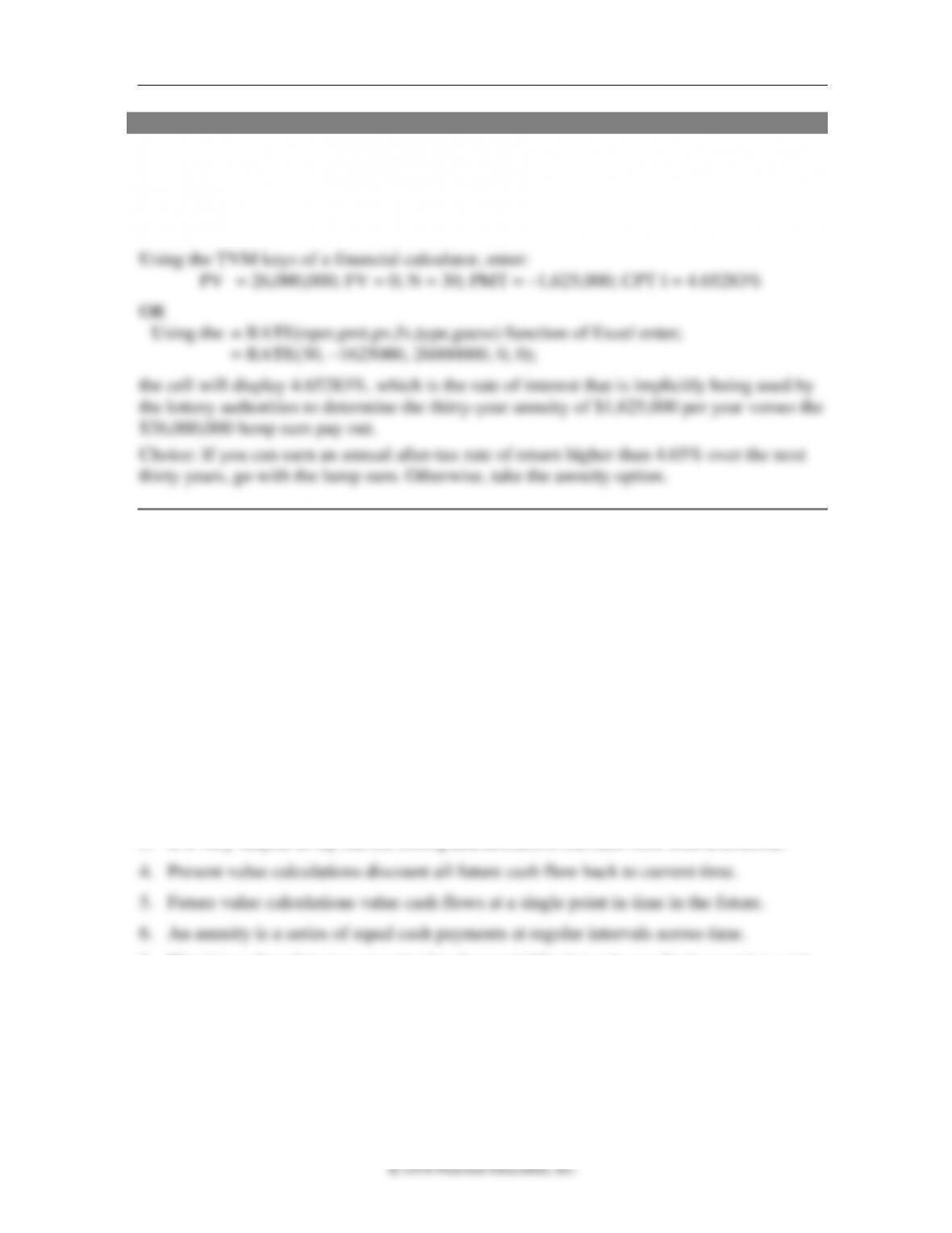
over the given number of years. If the winner feels that he or she can earn a higher after-tax
rate of return on the lump sum payout than the implied rate used by the authorities, the
lump sum choice would be better. Of course, as pointed out by the author, other factors are
being ignored here.
Chapter 4 ◼ The Time Value of Money (Part 2) 87
Example 9: Calculating an implied rate of return given an annuity
Let’s say that you have just won the state lottery. The authorities have given you a choice
of either taking a lump sum of $26,000,000 or a thirty-year annuity of $1,625,000. Both
payments are assumed to be after-tax. What will you do?
Calculate the implied interest rate given the lump sum and the thirty-year annuity
4.9 Ten Important Points
about the TVM Equation (Slides 4-42 to 4-44)
After covering the various topics dealing with the discounting and compounding of lump
sums and annuity streams in this two-part series, the author identifies ten key points that
students must remember going forward. It is important to advise students that a proper
grasp of these ten points is paramount to their success in dealing with more complex
financial problems that lie ahead.
Ten Key Points about Time Value of Money
1. Amounts of money can be added or subtracted only if they are at the same point in
time.
2. The timing and the amount of the cash flow are what matters.
3. It is very helpful to lay out the timing and amount of the cash flow with a timeline.
7. The time value of money equation has four variables but only one basic equation, and
so you must know three of the four variables before you can solve for the missing or
unknown variable.
8. There are three basic methods to solve for an unknown time value of money variable:
Method 1, using equations and calculating the answer; Method 2, using the TVM keys
on a calculator; and Method 3, using financial functions from a spreadsheet. All three
give the same answer because they all use the same time value of money equation.
© 2018 Pearson Education, Inc.
and (3) principal and interest as you go with equal and regular payments, or amortized
loans.
10. Despite the seemingly accurate answers from the time value of money equation, in
many situations we cannot classify all the important data into the variables of present
value time, interest rate, payment, and future value.
Questions
1. What is the difference between a series of payments and an annuity? What are the
two specific characteristics of a series of payments that make them an annuity?
An annuity is a series of payments of equal size at equal intervals. Uniform payments
values or at different intervals, it is not an annuity.
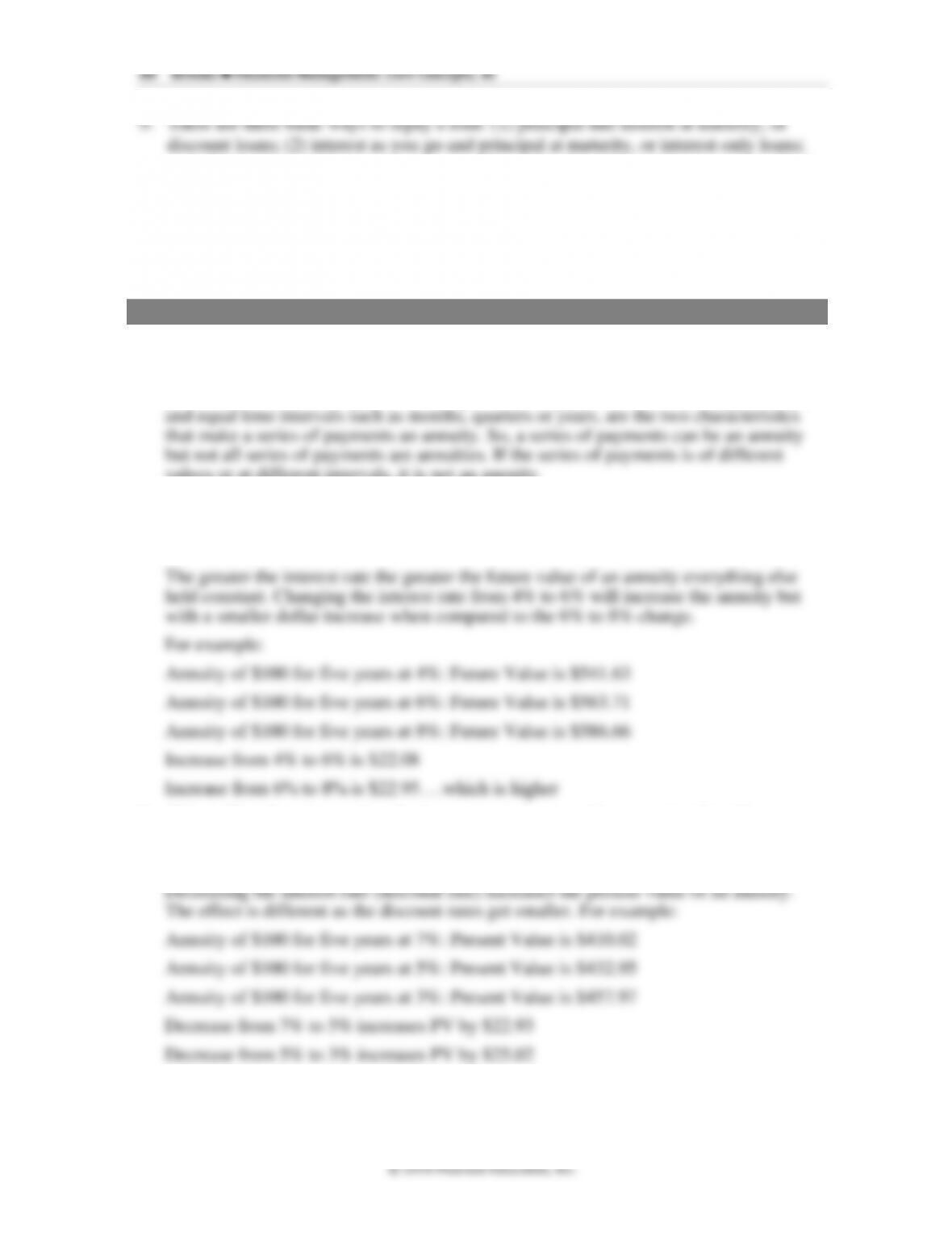
2. What effect does increasing the interest rate have on the future value of an
annuity? Does a change from 4% to 6% have the same dollar effect as a change
from 6% to 8%?
3. What effect does increasing the interest rate have on the present value of an
annuity? Does a decrease from 7% to 5% have the same dollar effect as a decrease
from 5% to 3%?
90 Brooks ◼ Financial Management: Core Concepts, 4e
Prepping for Exams
1. b.
2. b.
Problems
1. Different cash flow. Given the following cash inflow at the end of each year, what is
the future value of this cash flow at 6%, 9%, and 15% interest rates at the end of the
seventh year?
Year 1 $15,000
Year 2 $20,000
Year 3 $30,000
Years 4 through 6 $0
Year 7 $150,000
ANSWER

© 2018 Pearson Education, Inc.
6. Different cash flow. Given the following cash inflow, what is the present value of this
cash flow at 5%, 10%, and 25% discount rates?
Year 1: $3,000
Year 2: $5,000
Years 3 through 7: $0
Year 8: $25,000
ANSWER