
329
Cash Flow Chapter 10
Cash Flow Estimation
LEARNING OBJECTIVES (Slide 10-2)
1. Understand the importance of cash flow and the distinction between cash flow and profits.
2. Identify incremental cash flow.
3. Calculate depreciation and cost recovery.
4. Understand the cash flow associated with the disposal of depreciable assets.
5. Estimate incremental cash flow for capital budgeting decisions.
IN A NUTSHELL…
In this chapter, the author examines how cash flow differs from profits. Because cash flow is the
lifeline of business, it is very important to understand how to measure and forecast the various
sources of cash flow that arise from the investment and disposal of assets. Accordingly, topics
such as identifying and estimating incremental cash flow, calculating depreciation and cost
recovery, and adjusting for salvage and terminal values are covered as part of the steps
necessary prior to making capital budgeting decisions.
LECTURE OUTLINE
10.1 The Importance of Cash Flow (Slides 10-3 to 10-5)
Cash flow measures the actual inflow and outflow of cash, while profits represent merely an
accounting measure of periodic performance.
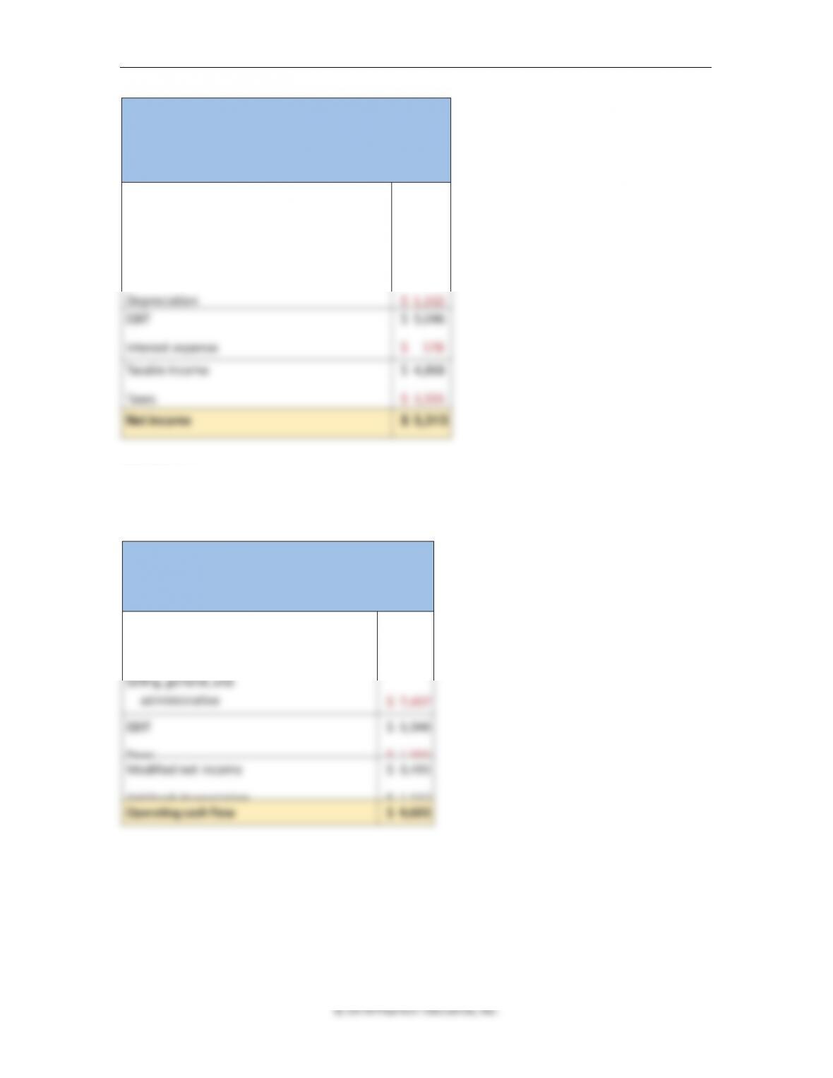
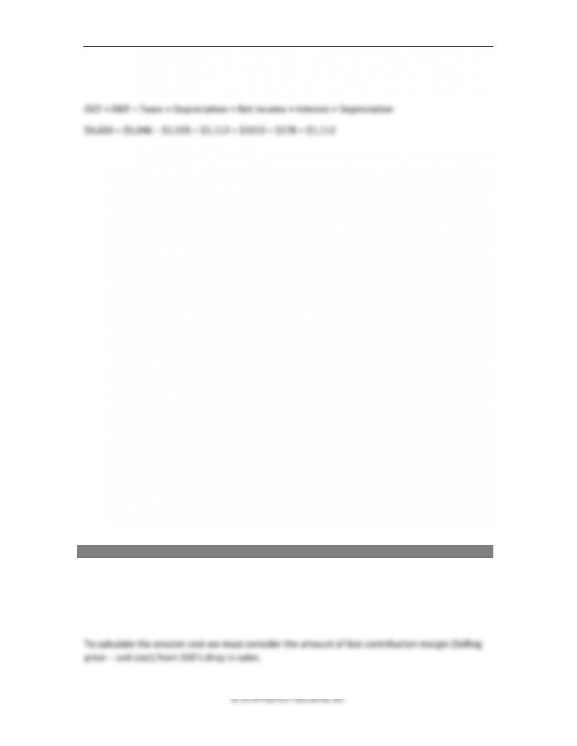
Figures 10.1 and 10.2 (shown next), help clarify the difference between net income and
operating cash flow (OCF) of a firm.
It is important to remind students that a firm can spend its operating cash flow but not its net
income.
Some firms have net losses (due to high depreciation write-offs) and yet can pay dividends from
cash balances, while others show profits and may not have the cash available.
Thus, cash flow is broader than net income as shown below.
330 Brooks ◼ Financial Management: Core Concepts, 4e
Cogswell Cola Company
Income
Statement
Year Ending December 31, 2017 ($
in
thousands)
Revenue
Cost of goods sold
Selling,
general, and
administrative expenses
Depreciation
$25,112
$11,497
$ 7,457
$ 1,112
EBIT
Interest expense
$ 5,046
$ 178
Taxable inc
om
e
Taxes
$ 4,868
$ 1,555
Net
incom
e
$ 3,313
FIGURE 10.1
Cogswell
Cola
Operating
Cash
Flow
Year Ending December 31, 2017
Revenue
Cost of goods sold
Selling,
general, and
administrative
$25,112
$11,497
$ 7,457
EBIT
Taxes
$ 5,046
$ 1,555
Modified net income
Add back depreciation
$ 3,491
$ 1,112
Operating cash
flow
$ 4,603
FIGURE 10.2
Figure 10.2 is a modified income statement in that it only considers the cash flow arising from
operations. Accordingly, interest expense (which is a financing cash flow) is not included, and
Chapter 10 ◼ Cash Flow Estimation 331
depreciation (which had been deducted in Figure 10.1, mainly for tax purposes) is added back.
Thus,
10.2 Estimating Cash Flow for
Projects: Incremental Cash Flow (Slides 10-6 to 10-14)
When a firm is considering either expanding a current line of business, starting a new venture,
or replacing an existing asset with a newer one, the changes in revenue and costs that occur will
have an incremental effect on its operating cash flow.
It is the timing and magnitude of these incremental cash flows that have to be carefully
estimated and evaluated as part of any capital budgeting analysis.
Seven important issues need to be tracked during a comprehensive cash flow estimation
process. These issues include sunk costs, opportunity cost, erosion, synergy gains, working
capital, capital expenditures, and depreciation or cost recovery of assets.
Sunk costs are expenses that have already been incurred, or that will be incurred, regardless of
the decision to accept or reject a project. For example, a marketing research study exploring
business possibilities in a region would be a sunk cost, since its expenditure has been done prior
to undertaking the project and will have to be paid whether or not the project is taken on. These
costs, although part of the income statement, should not be considered as part of the relevant
cash flows when evaluating a capital budgeting proposal.
Opportunity costs include costs that may not be directly observable or obvious, but result
from benefits being lost as a result of taking on a project. For example, if a firm decides to use
an idle piece of equipment as part of a new business, the value of the equipment that could be
realized by either selling or leasing it would be a relevant opportunity cost.
Erosion costs arise when a new product or service competes with revenue generated by a
current product or service offered by a firm. For example, if a store offers two types of photo–
copying services, a newer, more expensive choice and an older economical one, some of the
revenues from the older repeat customers will be lost and should therefore be accounted for in
the incremental cash flows.
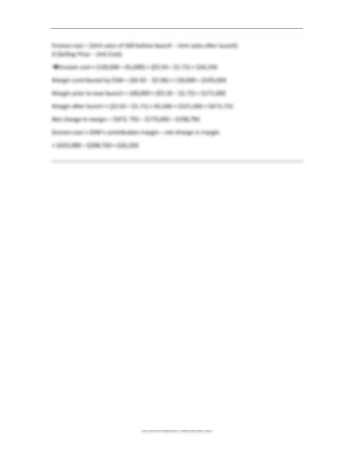
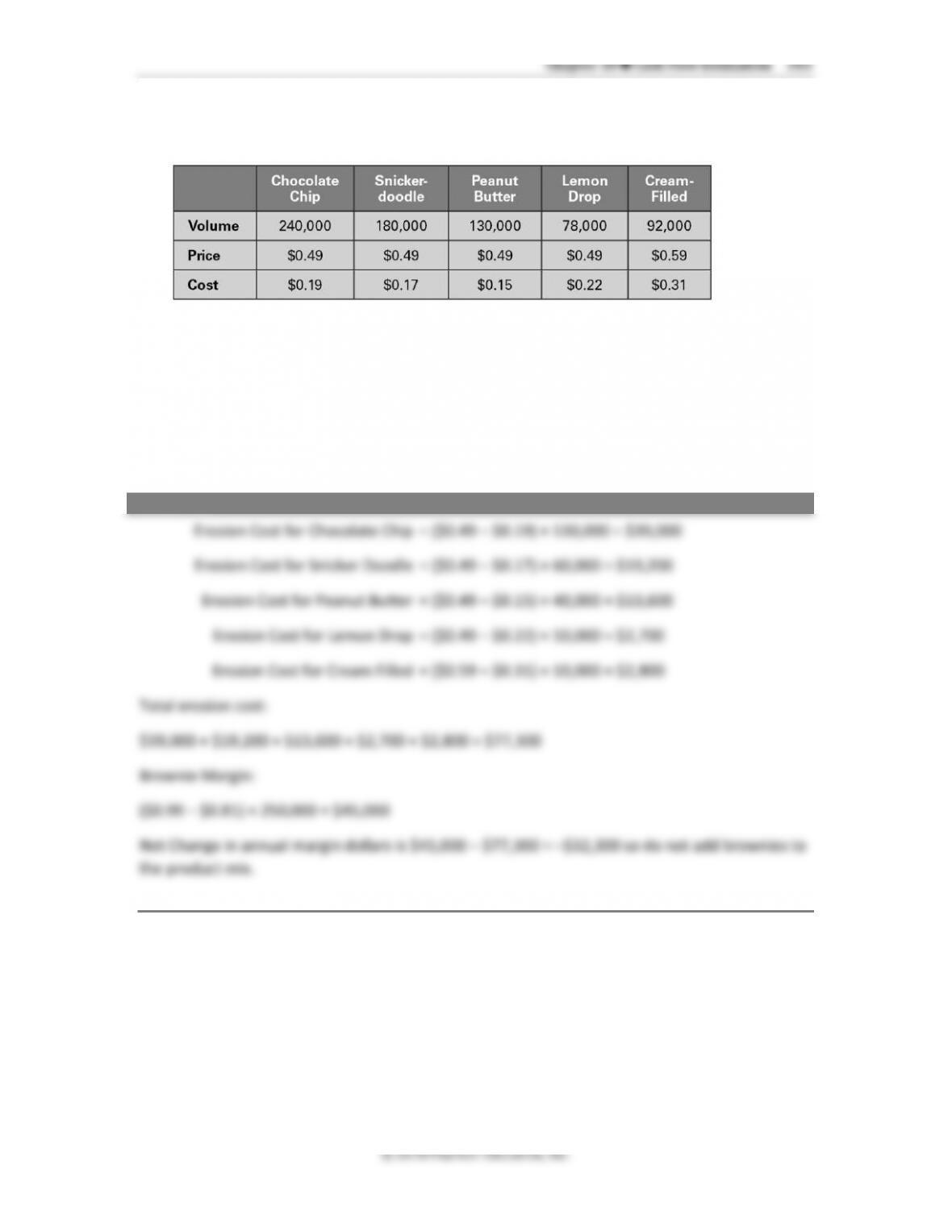
Example 1: Erosion costs
Frosty Desserts currently sell 100,000 of its Strawberry-Shortcake Delight each year for $3.50
per serving. Its cost per serving is $1.75. Its chef has come up with a newer, richer concoction,
“Extra–Creamy Strawberry Wonder,” which costs $2.00 per serving, will retail for $4.50 and
should bring in 130,000 customers. It is estimated that after the launch the sales for the original
variety will drop by 15%. Estimate the erosion cost associated with this venture.
332 Brooks ◼ Financial Management: Core Concepts, 4e
© 2018 Pearson Education, Inc.
Erosion cost = (Unit sales of SSD before launch – Unit sales after launch)
X (Selling Price – Unit Cost)
➔Erosion cost = (100,000 – 85,000) × ($3.50 – $1.75) = $26,250
Margin contributed by ESW = ($4.50 – $2.00) × 130,000 = $325,000
Margin prior to new launch = 100,000 × ($3.50 – $1.75) = $175,000
Margin after launch = ($3.50 – $1.75) × 85,000 + $325,000 = $473,750
Net change in margin = $473, 750 – $175,000 = $298,750
Erosion cost = ESW’s contribution margin – net change in margin
= $325,000 – $298,750 = $26,250

Chapter 10 ◼ Cash Flow Estimation 333
Synergy gains refer to the impulse purchases or sales increases for other existing products
related to the introduction of a new product. For example, if a gas station with a convenience
store attached adds a line of fresh donuts and bagels, the sales of coffee and milk would result
in synergy gains.
Working capital investment refers to the additional cash flows arising from changes in current
assets such as inventory and receivables (uses) and current liabilities such as accounts payables
(sources) that occur as a result of a new project.
Generally, at the end of the project, these additional cash flows are recovered and must be
accordingly shown as cash inflows.
Even though the net cash outflows—due to increase in net working capital at the start—may
equal the net cash inflow arising from the liquidation of the assets at the end, the time value of
money effects make these costs relevant.
10.3 Capital Spending and Depreciation (Slides 10-15 to 10-23)
When a firm spends capital to acquire a productive (depreciable) asset, it is allowed to expense
a portion of the cost of the asset each year, as a process of cost recovery via the reduced taxes
that result from the write-off.
The portion written off in the income statement each year is called the depreciation expense,
and the accumulated total kept track of in the balance sheet is known as accumulated
depreciation.
Thus, the book value of an asset equals its original cost less its accumulated depreciation.
We need to deal with depreciation when doing capital budgeting problems for two reasons:
(1) the tax flow implications from the operating cash flow and
(2) the gain or loss at disposal of a capital asset.
Firms have a choice of using either straight line depreciation rates, or modified accelerated cost
recovery system (MACRS) rates for allocating the annual depreciation expense, arising from an
asset acquisition.
Straight-line depreciation rates are easy to apply since the annual depreciation expense is
calculated by dividing the initial cost plus installation minus the expected residual value (at
termination) equally over the expected productive life of the asset. The annual depreciation
expenses are the same for each year.
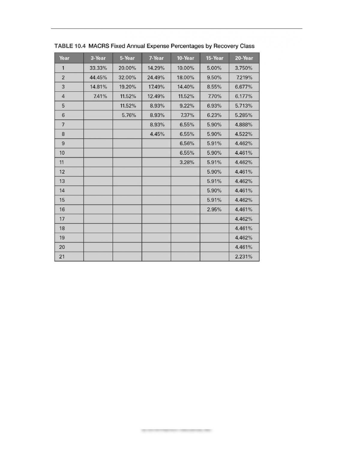
Modified accelerated cost recovery system rates were established by the federal
government in 1981 as a way to allow for firms to accelerate the depreciation write-off in early
years of the asset’s life.
These rates (shown below in Table 10.4) are set up based on various asset categories (class–
lives), as shown in Table 10.3 in the text.
334 Brooks ◼ Financial Management: Core Concepts, 4e
Each column relating to an asset life has one additional year of depreciation than the class-life
states, e.g., a three-year class life asset is depreciated over four years. This is because the
government assumes that the asset is put into use for only half a year at the start (half-year
convention), and thereby allowed ½ depreciation, with the last year (year four) being allowed
the balance required to reach 100% (which amounts to ½ the prior year’s percentage. The
depreciation rates in each column add up to 100%, i.e., no need to deduct residual value, with
higher rates being allowed in earlier years and less in later years.
With higher depreciation rates allowed in earlier years, the tax savings are higher due to the
time value of money.
Chapter 10 ◼ Cash Flow Estimation 335
Example 2: MACRS depreciation
The Grand Junction Furniture Company has just bought some specialty tools to be used in the
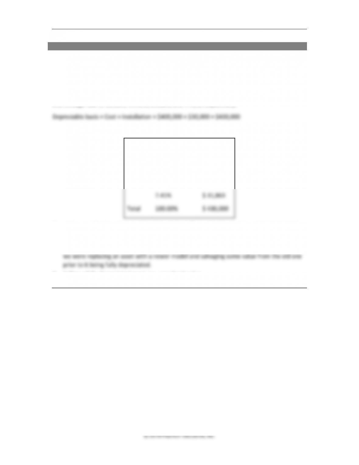
manufacture of high-end furniture. The cost of the equipment is $400,000 with an additional
$30,000 for installation. If the company has a marginal tax rate of 30%, compare its annual tax
savings that would be realized from using MACRS depreciation rates.
According to Table 10.3, specialty tools falls under a three-year class asset with rates in years
one through four of 33.33%, 44.45%, 14.81%, and 7.41%, respectively.
The annual depreciation expenses (i.e., annual rate × Dep. Basis) are shown below:
MACRS rate
Dep. Exp
33.33%
$ 143,319
44.45%
$ 191,135
14.81%
$ 63,683
7.41%
$ 31,863
Total
100.00%
$ 430,000
Two other specific depreciation-related issues that affect capital budgeting analysis include the
following:
1. Dealing with assets that are sold off prior to being fully depreciated, which would be true if
2. Selling a fully depreciated asset, i.e., zero book value.
10.4 Cash Flow and the Disposal
of Capital Equipment (Slides 10-24 to 10-27)
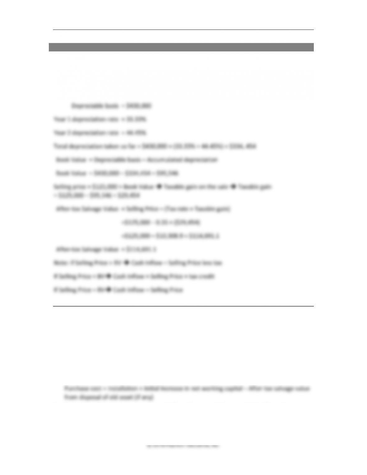
When a depreciable asset is sold, the cash inflow that results can be higher than, equal to, or
lower than the actual selling price of the asset, depending on whether it was sold above (taxable
gain), at (zero-gain), or below (tax credit) book value.
If the sale results in a taxable gain, then the cash inflow is reduced by the amount of the taxes
(Tax rate × (Selling Price – Book Value).
If the selling price is exactly equal to book value the cash inflow equals the sale price.
If the asset is sold below its book value, a loss results and can be written off taxes for the year,
resulting effectively in an addition to cash inflows equal to (Book Value-Selling Price) × Tax rate.
336 Brooks ◼ Financial Management: Core Concepts, 4e
Thus, the cash flow resulting from after-tax salvage value of a depreciable asset is calculated as
follows:
Chapter 10 ◼ Cash Flow Estimation 337
Example 3: Tax effects from disposal cash flow
Let’s say that the manager of the Grand Junction Furniture Company decides to dispose of the
specialty tools, acquired two years ago at a cost of $430,000 (including installation), to another
firm for $125,000. How much of an after-tax cash flow will result, assuming that the tools were
being depreciated based on the three-year MACRS rates and the company’s marginal tax rate is
35%
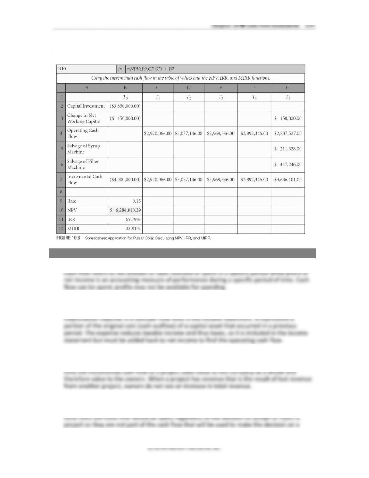
10.5 Projected Cash Flow for a New Product (Slides 10-28 to 10-35)
A comprehensive capital budgeting analysis requires the estimation of initial and future
incremental cash flows that are likely to result over the productive life of the project, followed
by the application of one or more of the evaluation techniques that were covered in Chapter 9.
In particular, the following four steps are typically involved:
1. Determination of the initial capital investment for the project
2. Estimation of the annual operating cash flows (incremental) generated by the project,
ignoring sunk costs and including erosion costs and side-effects. (Figures 10.3 through 10.5
in the text)
338 Brooks ◼ Financial Management: Core Concepts, 4e
© 2018 Pearson Education, Inc.
OCF = EBIT – Taxes + Depreciation
In the terminal year, besides the usual OCF we have to account for any salvage value that is
received, which requires the calculation of book value and taxes (or tax credits) on sale of
the asset (Table 10.7 in the text).
Terminal Year Cash flow = OCF + After-tax Salvage Value
3. Determination of the change in net working capital which is usually an increase (outflow) at
the beginning and a reduction (inflow) at the end.
(Table 10.7 in the text)
340 Brooks ◼ Financial Management: Core Concepts, 4e
© 2018 Pearson Education, Inc.
project. They are not wasted expenses because they may have been used to gather vital
information for the decision. For example, a market study to determine the potential market
of a new product may be critical in determining future sales and thus is important is
estimating future cash flow. However, the cost of the study is a sunk cost.
5. Give an example of an erosion cost. Explain why this cost is part of the incremental cash
flow of a project. Is there a case when a new product should get credit for additional
revenue of another already existing product?
Erosion cost is the lost profit of an existing product when a new product takes part of
6. Give an example of an opportunity cost, and explain how you would estimate the cost as
it applies to a particular project.
7. Why must a company typically invest in working capital when starting a new project? Why
is this investment in working capital recovered at the completion of the project?
Working capital is necessary for making a project go. For example, if you are introducing a
8. How does depreciation spread the capital expenditure of a project over the life of the
capital asset? Why is using MACRS usually beneficial to a company versus using straight–
line depreciation?
The original cost of new equipment or other large assets is not expensed on the income
9. Why is there typically a tax gain or tax loss at the disposal of capital assets?
Chapter 10 ◼ Cash Flow Estimation 341
© 2018 Pearson Education, Inc.
There is typically a tax gain or tax loss at the disposal of capital assets because it is rare that
the cash flow from the disposal is exactly equal to the current book value of the asset. The
book value is the original cost minus the accumulated depreciation.
10. All six decision models from Chapter 9 rely on the appropriate timing and amount of cash
flow. What are the potential errors a manager can make if this information is not
accurate?
Prepping for Exams
1. a.
Problems
1. Erosion costs. Fat Tire Bicycle Company currently sells 40,000 bicycles per year. The current
bike is a standard balloon-tire bike, selling for $90 with a production and shipping cost of
$35. The company is thinking of introducing an off-road bike with a projected selling price of
$410 and a production and shipping cost of $360. The projected annual sales are 12,000 off-
road bikes. The company will lose sales in fat-tire bikes of 8,000 units per year if it
introduces the new bike, however. What is the erosion cost from the new bike? Should Fat
Tire start producing the off-road bike?
ANSWER
344 Brooks ◼ Financial Management: Core Concepts, 4e
ANSWER
4. Opportunity cost. Richards’ Tree Farm, Inc. has branched into gardening over the years and
is now considering adding patio furniture to its product lineup. Currently, the area where
the patio furniture is to be displayed is a vacant slab of concrete attached to the indoor
shop. The company originally paid $8,500 to put in the slab of concrete three years ago. It
would now cost $12,000 to put in the same slab of concrete. Should Richards consider the
concrete slab when expanding its outdoor garden shop to include patio furniture? If yes,
which value should it use?
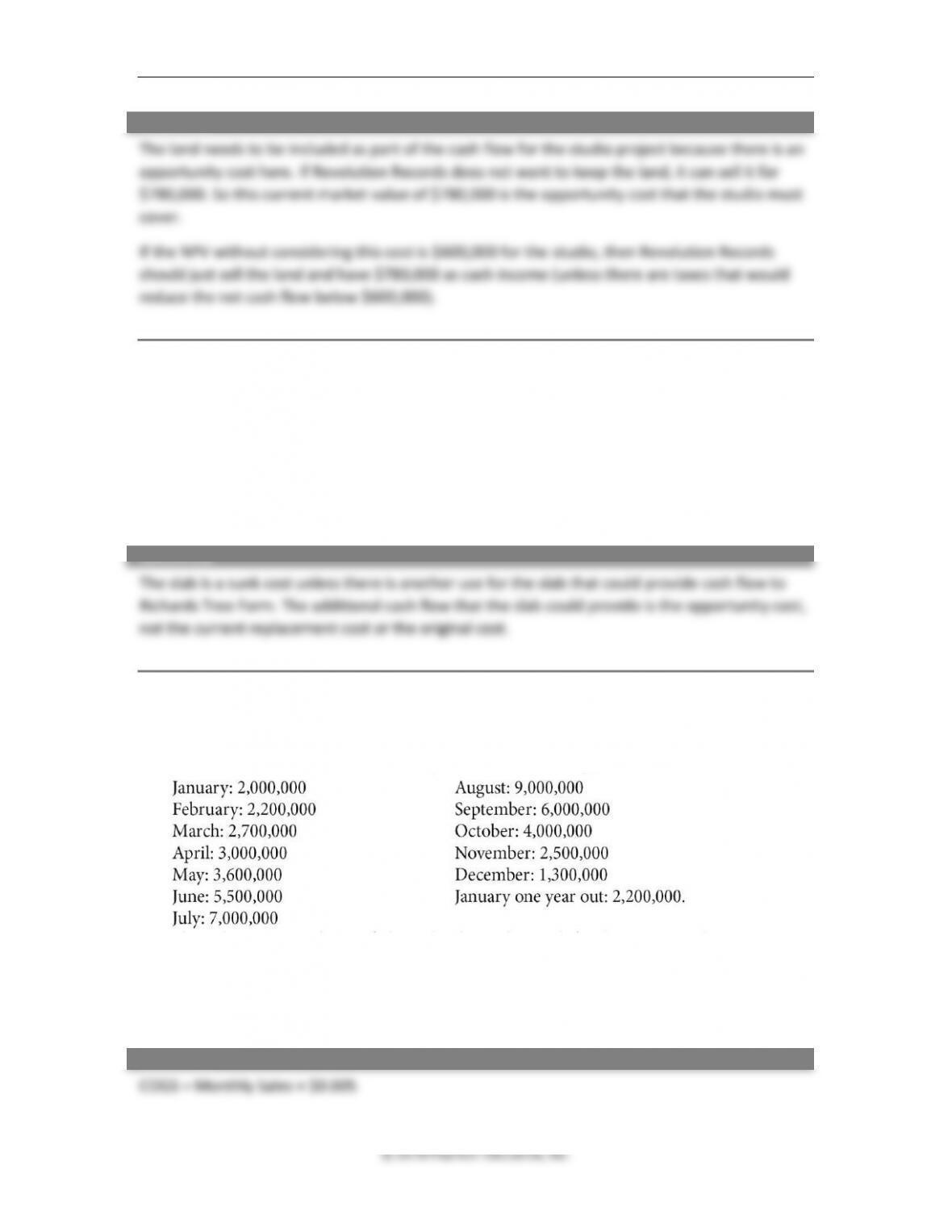
5. Working capital cash flow. Cool Water, Inc. sells bottled water. The firm keeps in inventory
plastic bottles at 10% of the monthly projected sales. These plastic bottles cost $0.005 each.
The monthly sales for the coming year are as follows:
Show the anticipated cost of plastic bottles each month for these projected sales, the
beginning inventory volume and ending inventory volume each month, and the monthly
increase or decrease in cash flow for inventory given that an increase is a use of cash and a
decrease is a source of cash.
ANSWER
Chapter 10 ◼ Cash Flow Estimation 345
© 2018 Pearson Education, Inc.
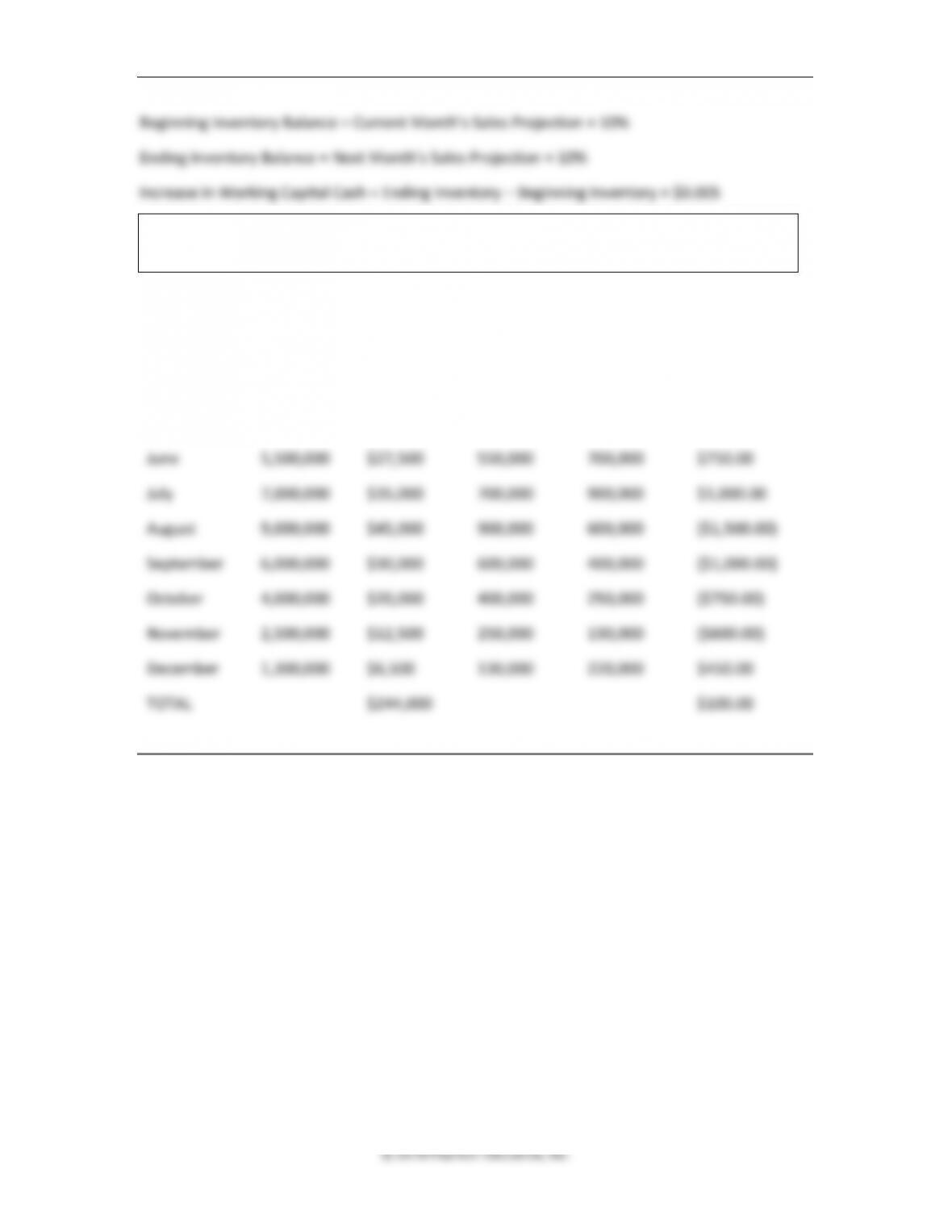
Beginning Inventory Balance = Current Month’s Sales Projection × 10%
Ending Inventory Balance = Next Month’s Sales Projection × 10%
Increase in Working Capital Cash = Ending Inventory – Beginning Inventory × $0.005
Month
Exp. Sales
(units)
Ant. COGS
Beg. Inv. Bal
End. Inv. Bal.
W. Cap.
Increase
January
2,000,000
$10,000
200,000
220,000
$100.00
February
2,200,000
$11,000
220,000
270,000
$250.00
March
2,700,000
$13,500
270,000
300,000
$150.00
April
3,000,000
$15,000
300,000
360,000
$300.00
May
3,600,000
$18,000
360,000
550,000
$950.00
June
5,500,000
$27,500
550,000
700,000
$750.00
July
7,000,000
$35,000
700,000
900,000
$1,000.00
August
9,000,000
$45,000
900,000
600,000
($1,500.00)
September
6,000,000
$30,000
600,000
400,000
($1,000.00)
October
4,000,000
$20,000
400,000
250,000
($750.00)
November
2,500,000
$12,500
250,000
130,000
($600.00)
December
1,300,000
$6,500
130,000
220,000
$450.00
TOTAL
$244,000
$100.00
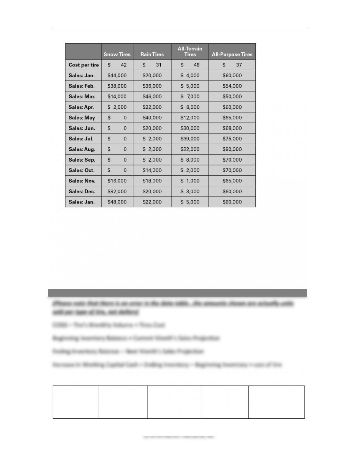
6. Working capital cash flow. Tires for Less is a franchise of tire stores throughout the greater
Northwest. It has projected the following unit sales per tire and costs of tires for the coming
year:
346 Brooks ◼ Financial Management: Core Concepts, 4e
The company policy is to have the next month’s anticipated sales for each tire type in the
warehouse. Shipments are made to the various stores throughout the Northwest from the
central warehouse. Show the anticipated cost of tires each month for these projected sales
by tire type, the beginning inventory volume and ending inventory volume each month for
each tire, and the monthly increase or decrease in cash flows for inventory given that an
increase is a use of cash and a decrease is a source of cash. Find the total cost of goods sold
and change in monthly working capital cash flows for all tires. What do you notice about the
working capital change when you combine all four tires?
ANSWER
SNOW TIRES
Month
Anticipated
COGS
Beginning
Inventory
Balance
Ending
Inventory
Balance
Working Capital
Increase
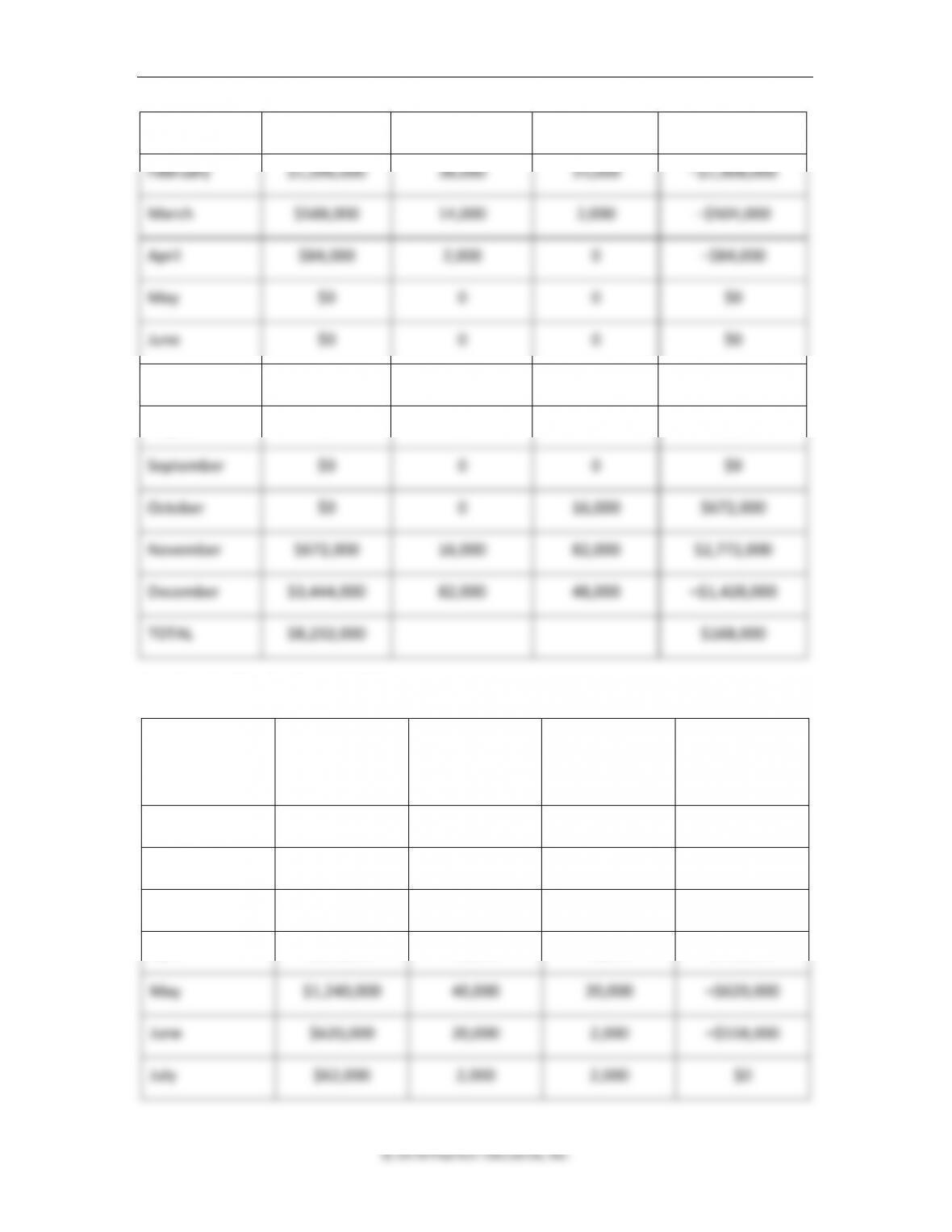
Chapter 10 ◼ Cash Flow Estimation 347
January
$1,848,000
44,000
38,000
–$252,000
February
$1,596,000
38,000
14,000
–$1,008,000
March
$588,000
14,000
2,000
–$504,000
April
$84,000
2,000
0
–$84,000
May
$0
0
0
$0
June
$0
0
0
$0
July
$0
0
0
$0
August
$0
0
0
$0
September
$0
0
0
$0
October
$0
0
16,000
$672,000
November
$672,000
16,000
82,000
$2,772,000
December
$3,444,000
82,000
48,000
–$1,428,000
TOTAL
$8,232,000
$168,000
Rain Tire Working Capital and COGS
Month
Anticipated
COGS
Beginning
Inventory
Balance
Ending
Inventory
Balance
Working Capital
Increase
January
$620,000
20,000
36,000
$496,000
February
$1,116,000
36,000
46,000
$310,000
March
$1,426,000
46,000
22,000
–$744,000
April
$682,000
22,000
40,000
$558,000
May
$1,240,000
40,000
20,000
–$620,000
June
$620,000
20,000
2,000
–$558,000
July
$62,000
2,000
2,000
$0
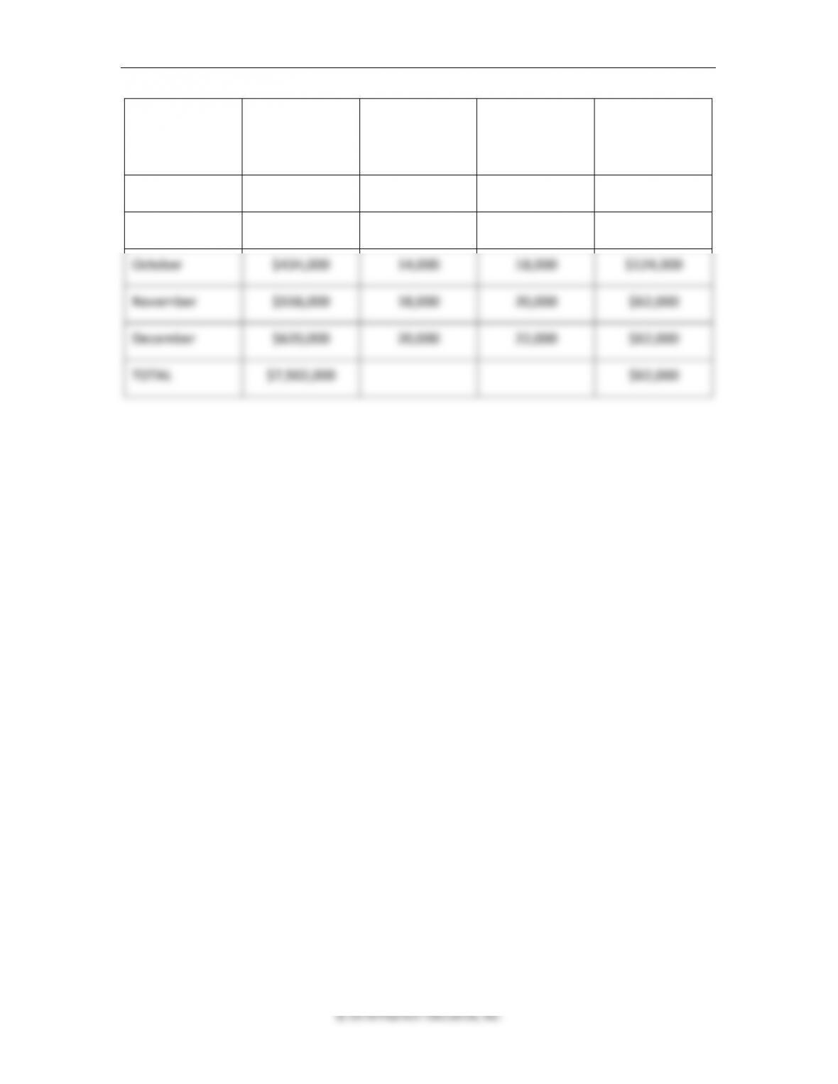
348 Brooks ◼ Financial Management: Core Concepts, 4e
Month
Anticipated
COGS
Beginning
Inventory
Balance
Ending
Inventory
Balance
Working Capital
Increase
August
$62,000
2,000
2,000
$0
September
$62,000
2,000
14,000
$372,000
October
$434,000
14,000
18,000
$124,000
November
$558,000
18,000
20,000
$62,000
December
$620,000
20,000
22,000
$62,000
TOTAL
$7,502,000
$62,000