978-0134663890 Chapter 12 Part 1

12-1$

Solutions)for)Chapter)12)–)Steady–State)Nonisothermal)

Reactor)Design$

)

P12-1)(a)))

(i)–(vii)$Individualized$solution$

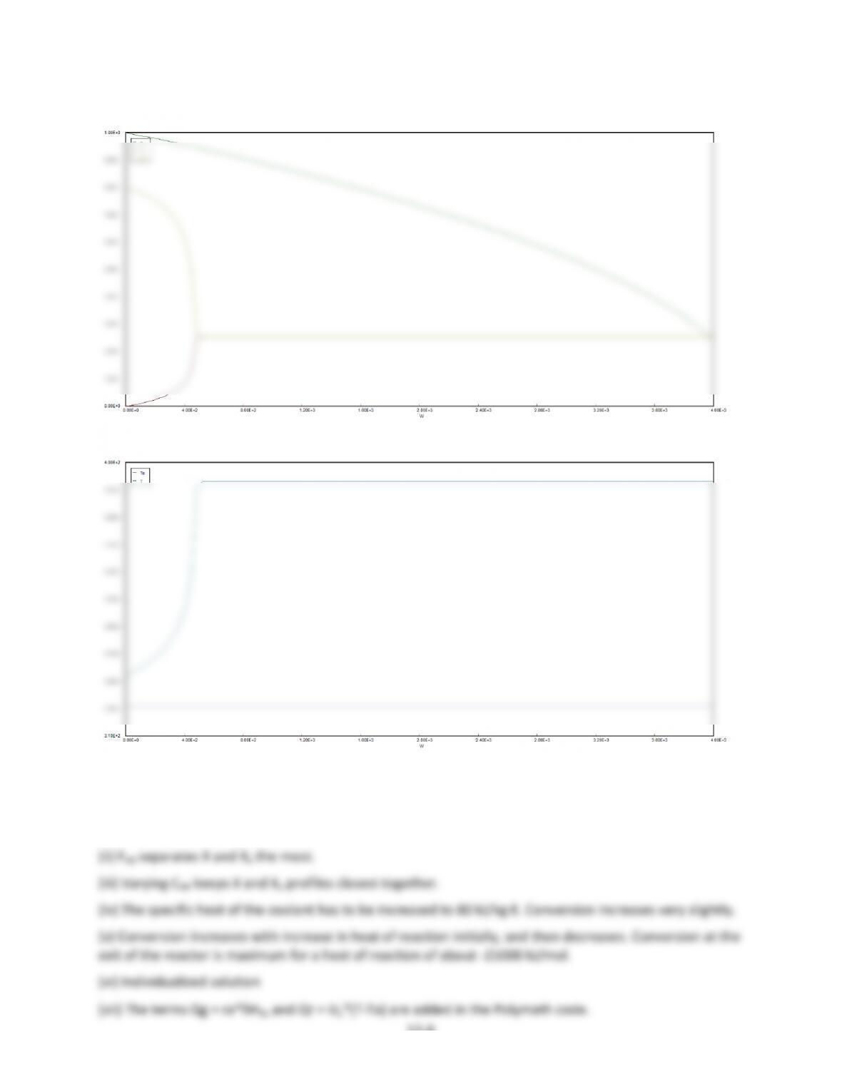
(viii)$They$separate$at$θI$=$1.1.$At$θI$=$1.2,$we$find$that$X$and$Xe$profiles$meet$at$low$α$but$separate$at$

(xii–xiv)$Individualized$solution$

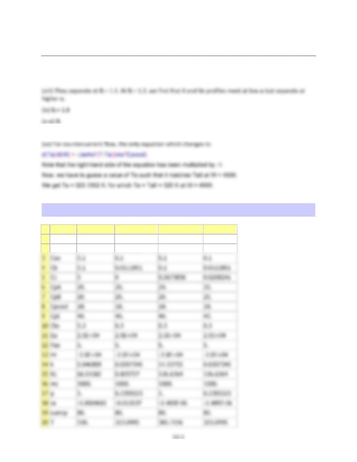
(xv)$For$countercurrent$flow,$the$only$equation$which$changes$is:$

See$Polymath$program$P12–1a–1.pol$

POLYMATH Report

Ordinary Differential Equations

Calculated values of DEQ variables

Variable

Initial value

Minimal value

Maximal value

Final value

1

alpha

0.0002

2

Ca

0.1

0.0111851

0.1

0.0111851

3

Cao

0.1

4

Cb

0.1

0.0111851

0.1

0.0111851

5

Cc

0

0.0673836

0.0258241

6

CpA

20.

7

CpB

20.

8

Cpcool

18.

9

CpI

40.

10

Cto

0.3

11

Ea

2.5E+04

12

Fao

5.

13

Hr

–2.0E+04

14

k

0.046809

0.0207345

11.53755

0.0207345

15

Kc

66.01082

0.805727

126.6264

16

mc

1000.

17

p

1.

0.2359323

1.

0.2359323

18

ra

–0.0004681

–0.012037

–2.485E–06

19

sumcp

80.

20

T

330.

323.0995

385.7156

323.0995

12-2$

21

Ta

323.1302

320.

323.1302

320.

22

thetaB

1.

23

thetaI

1.

24

To

330.

25

Uarho

0.5

26

W

0

4500.

27

X

0

0.5358329

28

Xe

0.8024634

0.3097791

0.849089

29

yao

0.3333333

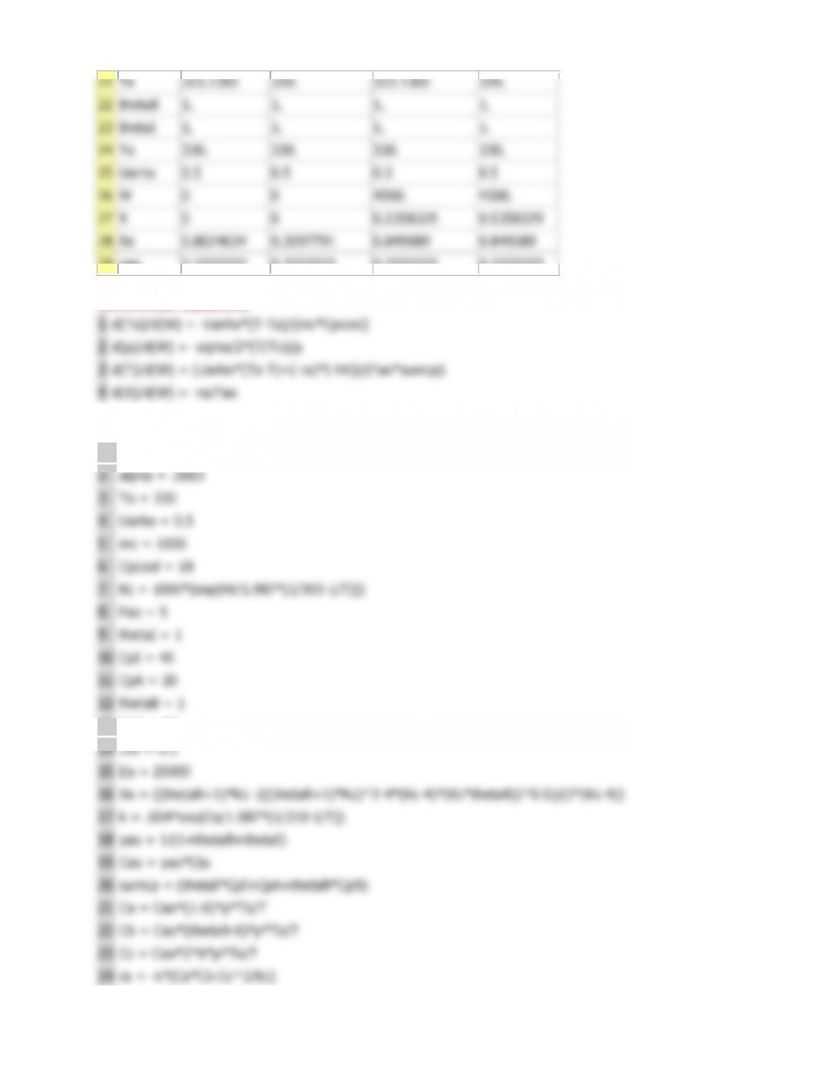
Differential equations

1

d(Ta)/d(W) = –Uarho*(T–Ta)/(mc*Cpcool)

2

d(p)/d(W) = –alpha/2*(T/To)/p

3

d(T)/d(W) = (Uarho*(Ta–T)+(–ra)*(–Hr))/(Fao*sumcp)

4

d(X)/d(W) = –ra/Fao

Explicit equations

1

Hr = –20000

2

alpha = .0002

3

To = 330

4

Uarho = 0.5

5

mc = 1000

6

Cpcool = 18

7

Kc = 1000*(exp(Hr/1.987*(1/303–1/T)))

8

Fao = 5

9

thetaI = 1

10

CpI = 40

11

CpA = 20

12

thetaB = 1

13

CpB = 20

14

Cto = 0.3

15

Ea = 25000

16

Xe = ((thetaB+1)*Kc– (((thetaB+1)*Kc)^2–4*(Kc–4)*(Kc*thetaB))^0.5)/(2*(Kc–4))

17

k = .004*exp(Ea/1.987*(1/310–1/T))

18

yao = 1/(1+thetaB+thetaI)

19

Cao = yao*Cto

20

sumcp = (thetaI*CpI+CpA+thetaB*CpB)

21

Ca = Cao*(1–X)*p*To/T

22

Cb = Cao*(thetaB–X)*p*To/T

23

Cc = Cao*2*X*p*To/T

24

ra = –k*(Ca*Cb–Cc^2/Kc)

$

12-3$

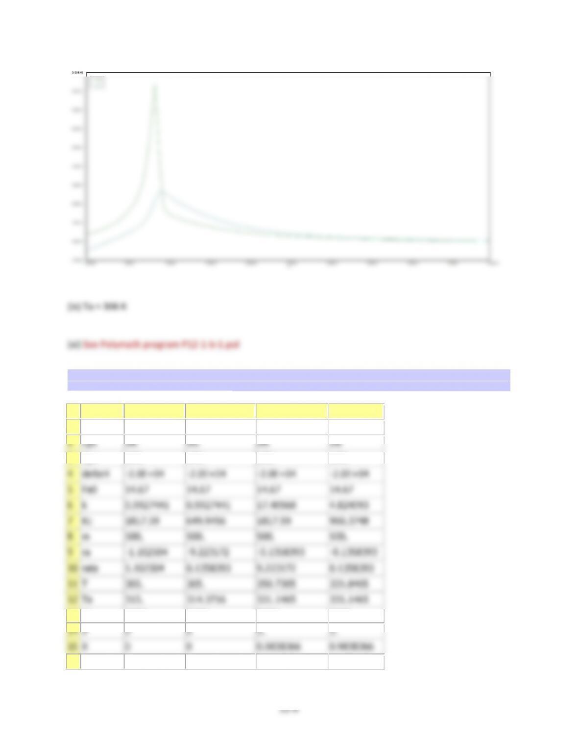
P12-1)(a))Continued$

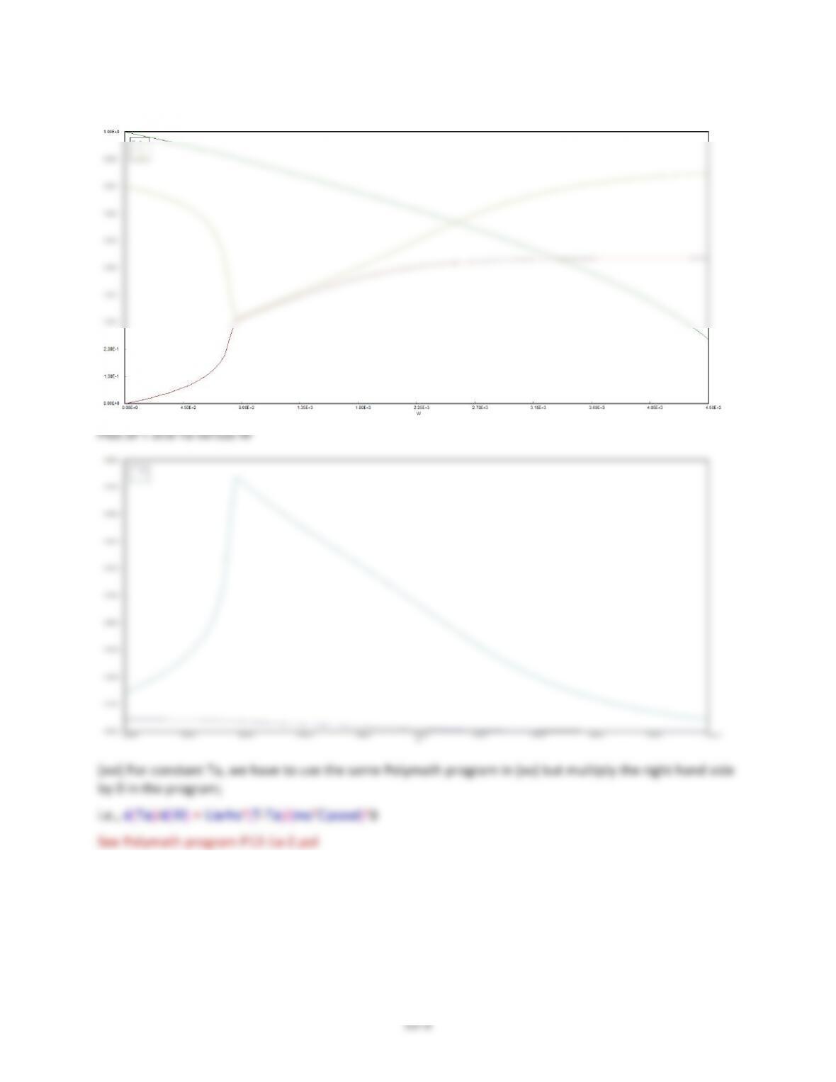
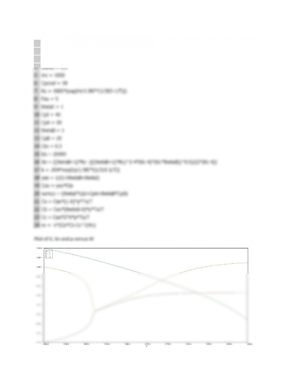
Plot$of$X,$Xe$and$p$versus$W$

$

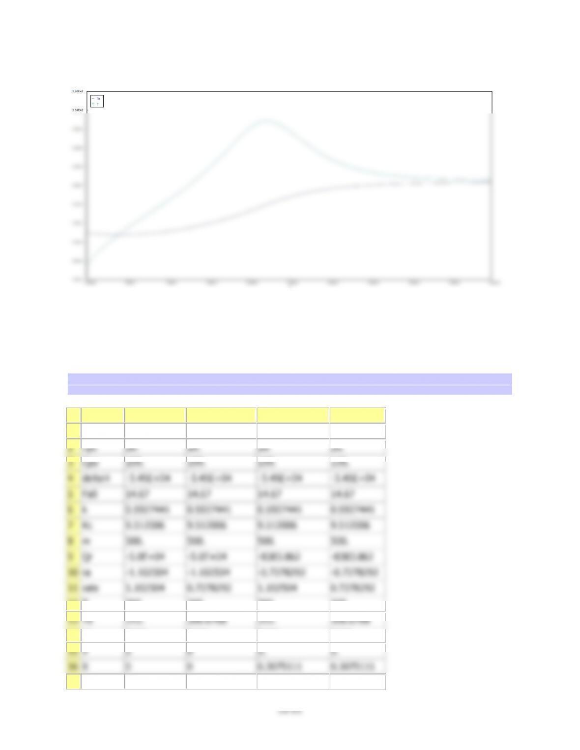
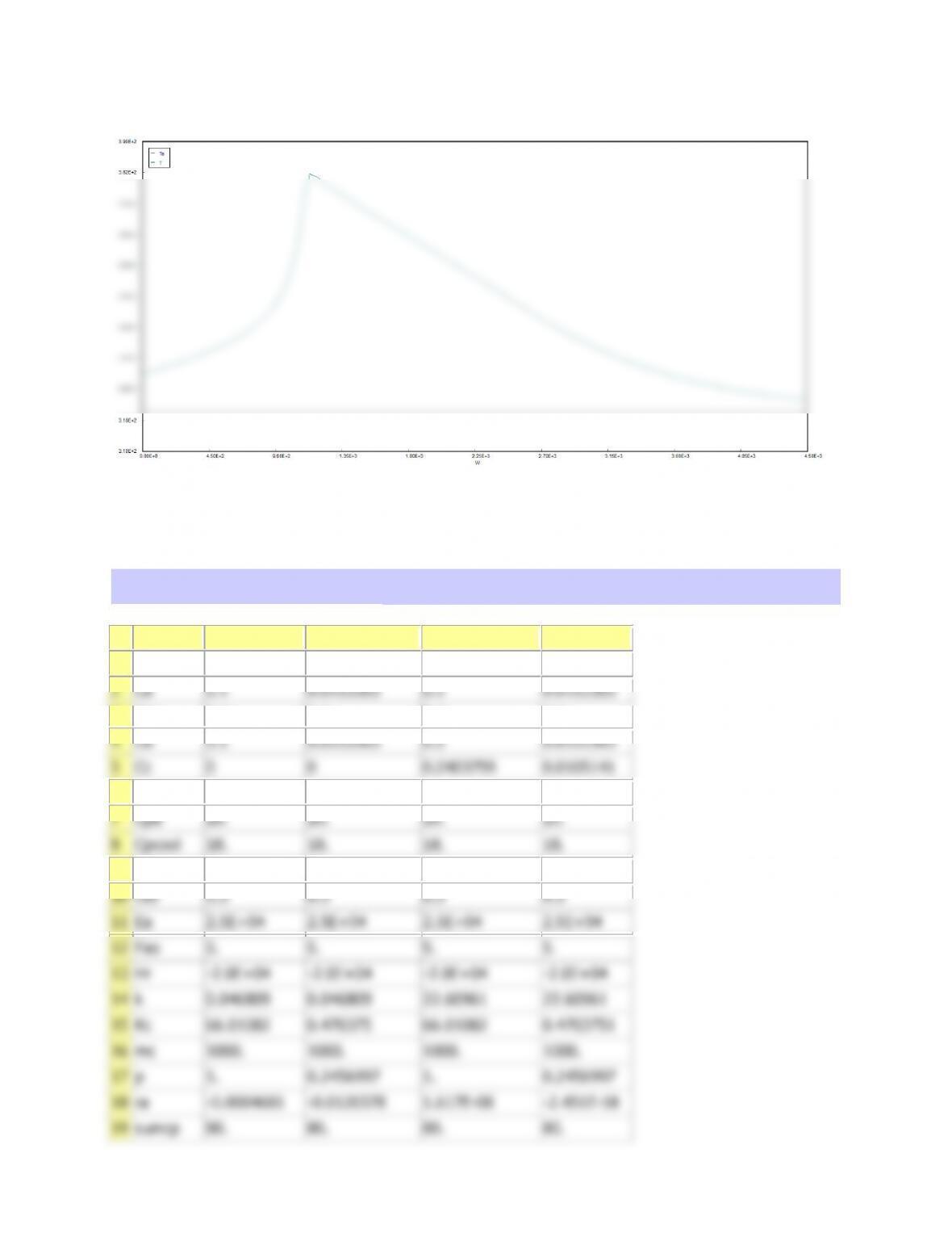
Plot$of$T$and$Ta$versus$W$

12-4$

P12-1)(a))Continued$

POLYMATH Report

Ordinary Differential Equations

Calculated values of DEQ variables

Variable

Initial value

Minimal value

Maximal value

Final value

1

alpha

0.0002

2

Ca

0.1

0.011675

0.1

0.011675

3

Cao

0.1

4

Cb

0.1

0.011675

0.1

0.011675

5

Cc

0

0.0659781

0.026488

6

CpA

20.

7

CpB

20.

8

Cpcool

18.

9

CpI

40.

10

Cto

0.3

11

Ea

2.5E+04

12

Fao

5.

13

Hr

–2.0E+04

14

k

0.046809

0.021188

8.254819

0.021188

15

Kc

66.01082

1.053204

124.4536

16

mc

1000.

17

p

1.

0.2441145

1.

0.2441145

18

ra

–0.0004681

–0.0080133

–2.769E–06

19

sumcp

80.

20

T

330.

323.2791

381.7968

323.2791

21

Ta

320.

22

thetaB

1.

23

thetaI

1.

24

To

330.

25

Uarho

0.5

26

W

0

4500.

27

X

0

0.5314832

28

Xe

0.8024634

0.3391177

0.8479767

29

yao

0.3333333

Differential equations

1

d(Ta)/d(W) = –Uarho*(T–Ta)/(mc*Cpcool) *0

2

d(p)/d(W) = –alpha/2*(T/To)/p

3

d(T)/d(W) = (Uarho*(Ta–T)+(–ra)*(–Hr))/(Fao*sumcp)

4

d(X)/d(W) = –ra/Fao

12-5$

P12-1)(a))Continued$

Explicit equations

1

Hr = –20000

2

alpha = .0002

3

To = 330

4

Uarho = 0.5

5

mc = 1000

6

Cpcool = 18

7

Kc = 1000*(exp(Hr/1.987*(1/303–1/T)))

8

Fao = 5

9

thetaI = 1

10

CpI = 40

11

CpA = 20

12

thetaB = 1

13

CpB = 20

14

Cto = 0.3

15

Ea = 25000

16

Xe = ((thetaB+1)*Kc– (((thetaB+1)*Kc)^2–4*(Kc–4)*(Kc*thetaB))^0.5)/(2*(Kc–4))

17

k = .004*exp(Ea/1.987*(1/310–1/T))

18

yao = 1/(1+thetaB+thetaI)

19

Cao = yao*Cto

20

sumcp = (thetaI*CpI+CpA+thetaB*CpB)

21

Ca = Cao*(1–X)*p*To/T

22

Cb = Cao*(thetaB–X)*p*To/T

23

Cc = Cao*2*X*p*To/T

24

ra = –k*(Ca*Cb–Cc^2/Kc)

)

Plot$of$X,$Xe$and$p$versus$W$

$

12-6$

P12-1)(a))Continued$

Plot$of$T$and$Ta$versus$W$

$

Ta$will$remain$constant$with$W$

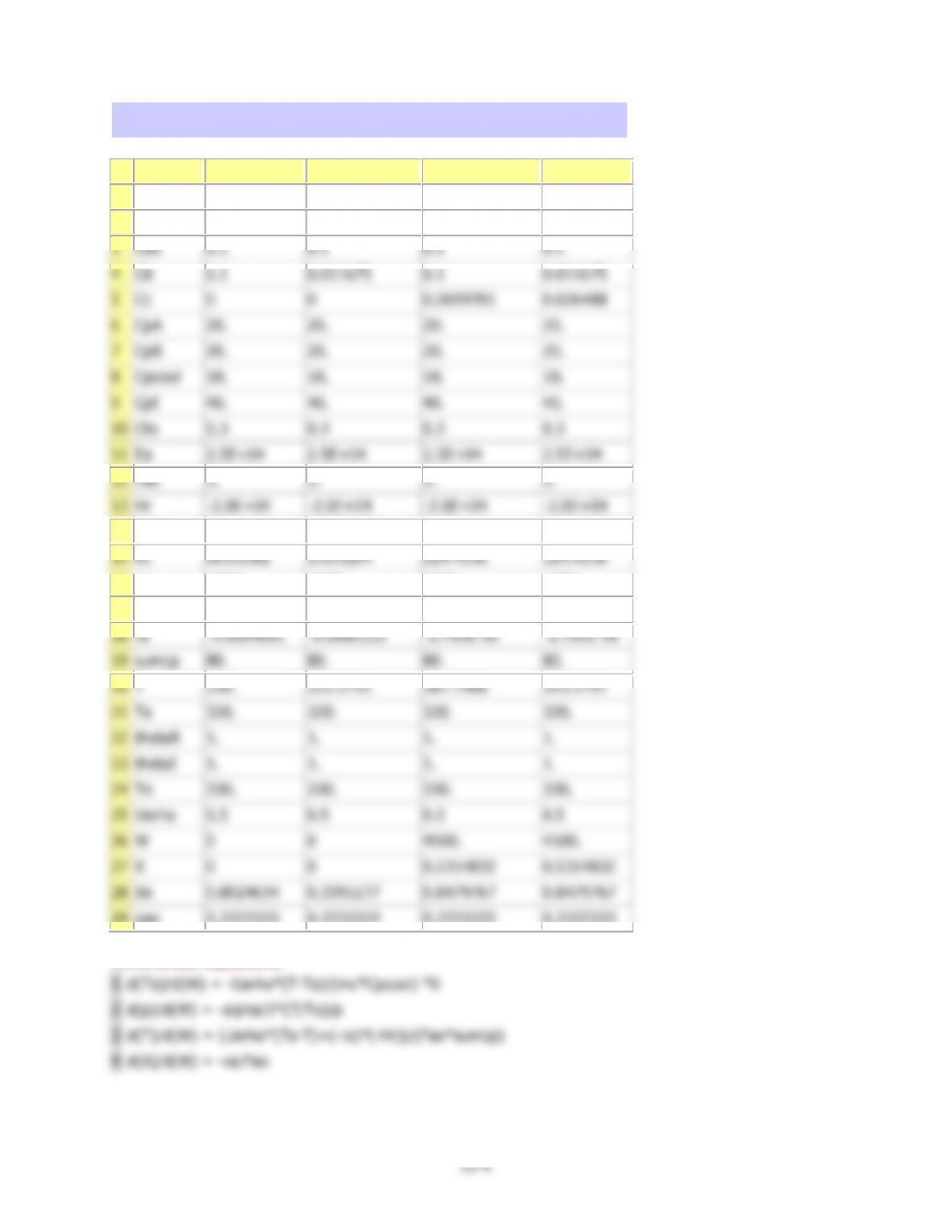
For$adiabatic$operation,$

Using$the$Polymath$program$of$part$(xv)$and$making$the$parameter$Ua$=0;$we$have;$

See$Polymath$program$P12–1a–3.pol$

POLYMATH Report

Ordinary Differential Equations

Calculated values of DEQ variables

Variable

Initial value

Minimal value

Maximal value

Final value

1

alpha

0.0002

2

Ca

0.1

0.0153303

0.1

0.0153303

3

Cao

0.1

4

Cb

0.1

0.0153303

0.1

0.0153303

5

Cc

0

0.0403759

0.0105141

6

CpA

20.

7

CpB

20.

8

Cpcool

18.

9

CpI

40.

10

Cto

0.3

11

Ea

2.5E+04

12

Fao

5.

13

Hr

–2.0E+04

14

k

0.046809

22.60961

15

Kc

66.01082

0.470375

66.01082

0.4703751

16

mc

1000.

17

p

1.

0.2456997

1.

0.2456997

18

ra

–0.0004681

–0.0120578

1.617E–08

–2.451E–18

19

sumcp

80.

12-7$

20

T

330.

393.8384

21

Ta

320.

22

thetaB

1.

23

thetaI

1.

24

To

330.

25

Uarho

0

26

W

0

4000.

27

X

0

0.2553537

28

Xe

0.8024634

0.2553537

0.8024634

0.2553537

29

yao

0.3333333

1

d(Ta)/d(W) = –Uarho*(T–Ta)/(mc*Cpcool) *0

2

d(p)/d(W) = –alpha/2*(T/To)/p

3

d(T)/d(W) = (Uarho*(Ta–T)+(–ra)*(–Hr))/(Fao*sumcp)

4

d(X)/d(W) = –ra/Fao

$

Explicit equations

1

Hr = –20000

2

alpha = .0002

3

To = 330

4

Uarho = 0

5

mc = 1000

6

Cpcool = 18

7

Kc = 1000*(exp(Hr/1.987*(1/303–1/T)))

8

Fao = 5

9

thetaI = 1

10

CpI = 40

11

CpA = 20

12

thetaB = 1

13

CpB = 20

14

Cto = 0.3

15

Ea = 25000

16

Xe = ((thetaB+1)*Kc– (((thetaB+1)*Kc)^2–4*(Kc–4)*(Kc*thetaB))^0.5)/(2*(Kc–4))

17

k = .004*exp(Ea/1.987*(1/310–1/T))

18

yao = 1/(1+thetaB+thetaI)

19

Cao = yao*Cto

20

sumcp = (thetaI*CpI+CpA+thetaB*CpB)

21

Ca = Cao*(1–X)*p*To/T

22

Cb = Cao*(thetaB–X)*p*To/T

23

Cc = Cao*2*X*p*To/T

24

ra = –k*(Ca*Cb–Cc^2/Kc)

$

12-8$

P12-1)(a))Continued$

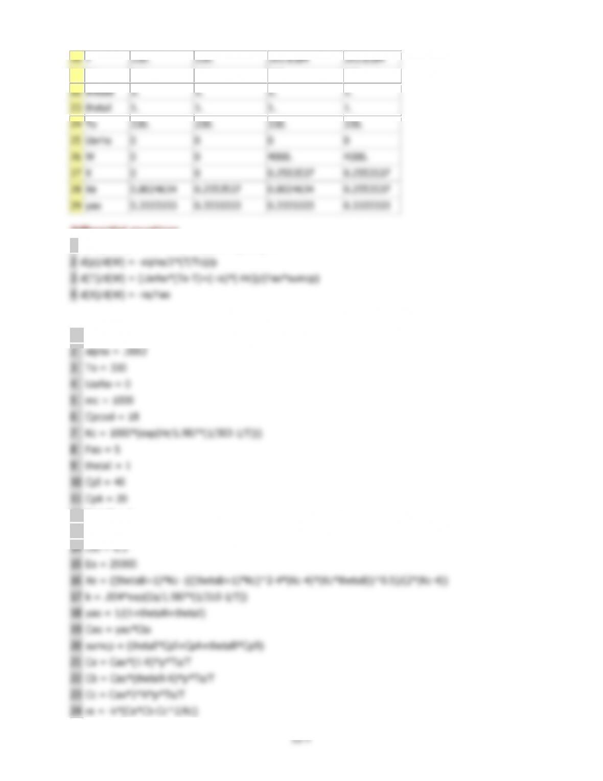
Plot$of$X,$Xe$and$p$versus$W;$

$

Plot$of$T$and$Ta$versus$W$

$

Ta$remains$a$constant$

$

P12-1)(b))

(i)$Ua$brings$the$temperature$profiles$close$together.$

(ii)$FA0$separates$X$and$Xe$the$most.$

12-9$

P12-1)(b))Continued$

$

(viii)$Individualized$solution$

(ix)$Ta$=$306$K$

(x)$Individualized$solution$

(xi)$See$Polymath$program$P12-1-b–1.pol$

POLYMATH Report

Ordinary Differential Equations

Calculated values of DEQ variables

Variable

Initial value

Minimal value

Maximal value

Final value

1

Ca0

1.86

2

Cpc

28.

3

Cpo

159.

4

deltaH

–2.0E+04

5

Fa0

14.67

6

k

0.5927441

17.40568

4.824093

7

Kc

1817.59

649.9456

1817.59

960.3748

8

m

500.

9

ra

–1.102504

–9.223172

–0.1358393

10

rate

1.102504

0.1358393

9.223172

0.1358393

11

T

305.

350.7305

331.8405

12

Ta

315.

314.3716

331.1465

13

Ua

5000.

14

V

0

5.

15

X

0

0.9838366

16

Xe

0.9994501

0.9984638

0.9994501

0.9989598

)

12–10$

P12-1)(b))Continued$

Differential equations

1

d(Ta)/d(V) = Ua*(T–Ta)/m/Cpc

2

d(X)/d(V) = –ra/Fa0

3

d(T)/d(V) = ((ra*deltaH)–Ua*(T–Ta))/Cpo/Fa0

Explicit equations

1

Cpc = 28

2

m = 500

3

Ua = 5000

4

Ca0 = 1.86

5

Fa0 = 0.9*163*.1

6

deltaH = –20000

7

k = 31.1*exp((7906)*(T–360)/(T*360))

8

Kc = 1000*exp((deltaH/8.314)*((T–330)/(T*330)))

9

Xe = Kc/(1+Kc)

10

ra = –k*Ca0*(1–(1+1/Kc)*X)

11

Cpo = 159

12

rate = –ra

$

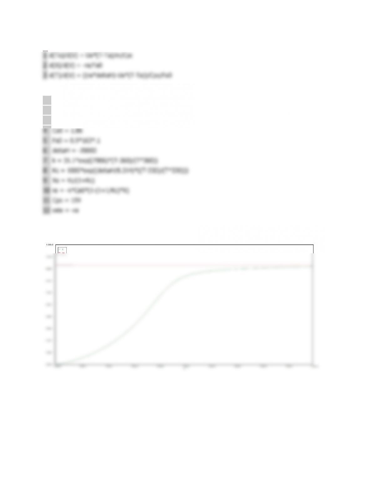
Plot$of$X$and$Xe$versus$V$

$

12–11$

P12-1)(b))Continued$

Plot$of$T$and$Ta$versus$V$

$

(xii)$For$isothermal$operation,$the$same$code$in$part$(vii)$is$used,$with$one$change:$

d(T)/d(V) = ((ra*deltaH)–Ua*(T–Ta))/Cpo/Fa0*0

Note$that$the$right$hand$side$of$the$equation$is$multiplied$by$0.$

See$Polymath$program$P12-1-b-2.pol$

POLYMATH Report

Ordinary Differential Equations

Calculated values of DEQ variables

Variable

Initial value

Minimal value

Maximal value

Final value

1

Ca0

1.86

2

Cpc

28.

3

Cpo

159.

4

deltaH

–3.45E+04

5

Fa0

14.67

6

k

0.5927441

7

Kc

9.512006

8

m

500.

9

Qr

–5.0E+04

–8383.862

10

ra

–1.102504

–0.7278292

11

rate

1.102504

0.7278292

1.102504

0.7278292

12

T

305.

13

Ta

315.

306.6768

315.

306.6768

14

Ua

5000.

15

V

0

5.

16

X

0

0.3075111

17

Xe

0.9048707

12–12$

P12–1)(b))Continued

Differential equations

1

d(Ta)/d(V) = Ua*(T–Ta)/m/Cpc

2

d(X)/d(V) = –ra/Fa0

3

d(T)/d(V) = ((ra*deltaH)–Ua*(T–Ta))/Cpo/Fa0*0

Explicit equations

1

Cpc = 28

2

m = 500

3

Ua = 5000

4

Ca0 = 1.86

5

Fa0 = 0.9*163*.1

6

deltaH = –34500

7

k = 31.1*exp((7906)*(T–360)/(T*360))

8

Kc = 3.03*exp((deltaH/8.314)*((T–333)/(T*333)))

9

Xe = Kc/(1+Kc)

10

ra = –k*Ca0*(1–(1+1/Kc)*X)

11

Cpo = 159

12

rate = –ra

13

Qr = Ua*(T–Ta)

)

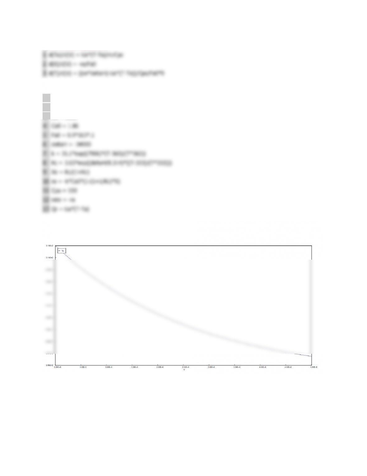
Plot$of$Ta$versus$V$to$maintain$isothermal$operation$

$

12–13$

P12-1)(b))Continued$$

Plot$of$Qr$versus$V$to$maintain$isothermal$operation$

$

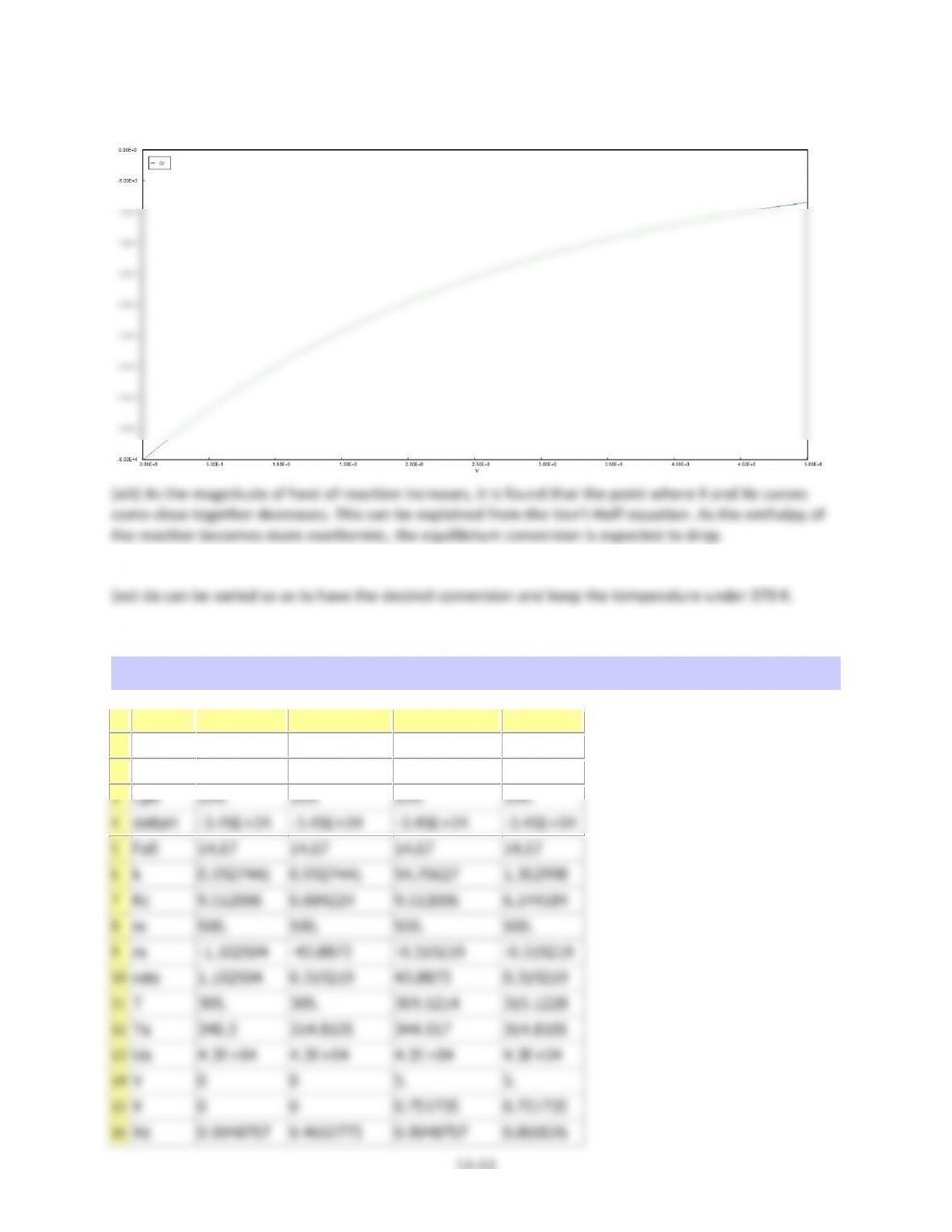
(xiv)$No$solution$will$be$provided$

(xv)$Ua$can$be$varied$so$as$to$have$the$desired$conversion$and$keep$the$temperature$under$370$K.$$

See$Polymath$program$P12-1-b-3.pol$

$

POLYMATH Report

Ordinary Differential Equations

Calculated values of DEQ variables

Variable

Initial value

Minimal value

Maximal value

Final value

1

Ca0

1.86

2

Cpc

28.

3

Cpo

159.

4

deltaH

–3.45E+04

5

Fa0

14.67

6

k

0.5927441

54.76627

1.362998

7

Kc

9.512006

0.884224

9.512006

6.144184

8

m

500.

9

ra

–1.102504

–43.8873

–0.319219

10

rate

1.102504

0.319219

43.8873

0.319219

11

T

305.

369.5214

315.1228

12

Ta

340.3

314.8105

344.917

314.8105

13

Ua

4.3E+04

14

V

0

5.

15

X

0

0.751735

16

Xe

0.9048707

0.4692775

0.9048707

0.860026

12–14$

P12-1)(b))Continued$$

Differential equations

1

d(Ta)/d(V) = –Ua*(T–Ta)/m/Cpc

2

d(X)/d(V) = –ra/Fa0

3

d(T)/d(V) = ((ra*deltaH)–Ua*(T–Ta))/Cpo/Fa0

Explicit equations

1

Cpc = 28

2

m = 500

3

Ua = 43000

4

Ca0 = 1.86

5

Fa0 = 0.9*163*.1

6

deltaH = –34500

7

k = 31.1*exp((7906)*(T–360)/(T*360))

8

Kc = 3.03*exp((deltaH/8.314)*((T–333)/(T*333)))

9

Xe = Kc/(1+Kc)

10

ra = –k*Ca0*(1–(1+1/Kc)*X)

11

Cpo = 159

12

rate = –ra

$

In$the$above$report,$it$can$be$seen$that$Ua$is$the$only$changed$parameter$to$get$a$conversion$that$is$

greater$than$75%$and$the$temperature$is$maintained$under$370$K.$$

$

P12-1$(c)$

(i)$The$reaction$dies$out$near$the$reactor$entrance$when$varying$the$heat$capacity$of$A.$

(v)$Individualized$solution$

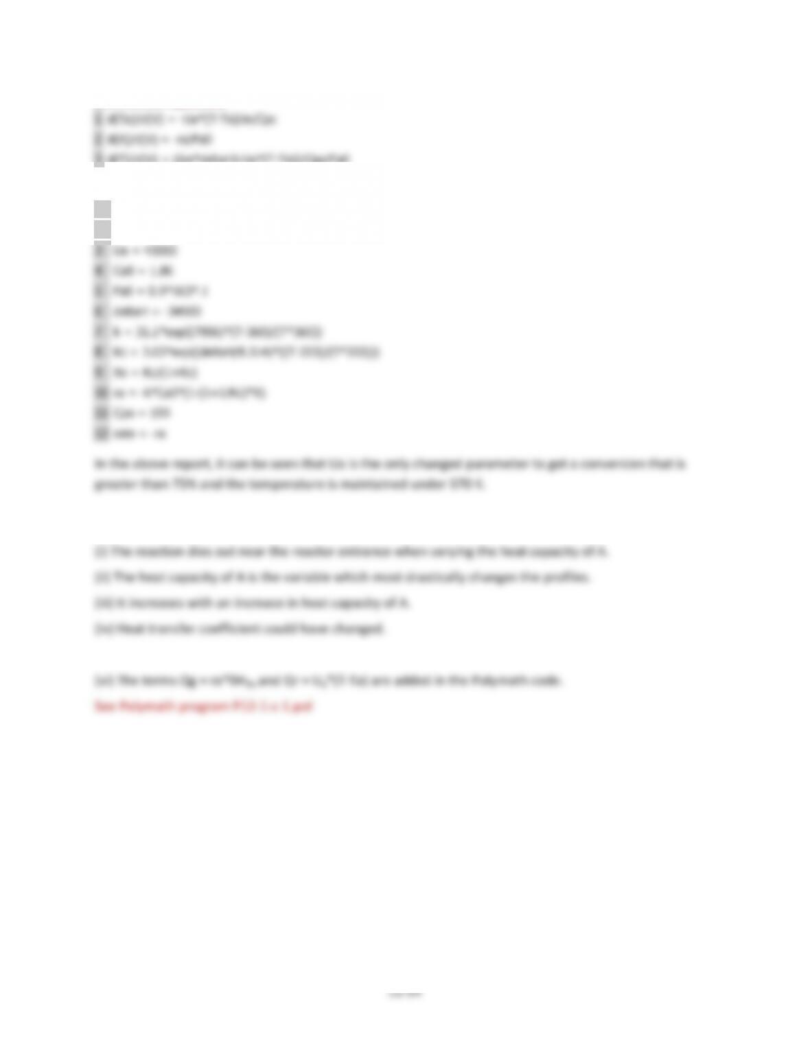
(vi)$The$terms$Qg$=$ra*δHRx$and$Qr$=$Ua*(T–Ta)$are$added$in$the$Polymath$code.$

12–15$

P12-1)(c))Continued$

Case1:))adiabatic)operation$

Qr=0$in$this$case$$$

$

Case)2:)For)constant)heat)exchange)conditions$

$

12–16$

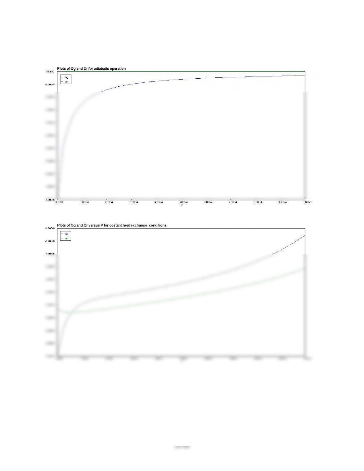
Case)3:)Co–current)heat)exchange)$

$

Case)4):)counter)current)heat)exchange):)

We$$need$to$guess$a$value$of$Ta$such$that$at$exit$Ta$=$1250K$

If$we$take$Ta(0)$=$995.15K$then$this$can$be$done.$

$

(vii)$Now,$V$=$0.5$m3)

T0$=$1050$K$

Case)1:$adiabatic$operation;$

Substitute;$Ua$=$0$in$the$Polymath$code$

12–17$

P12-1)(c))Continued$

$

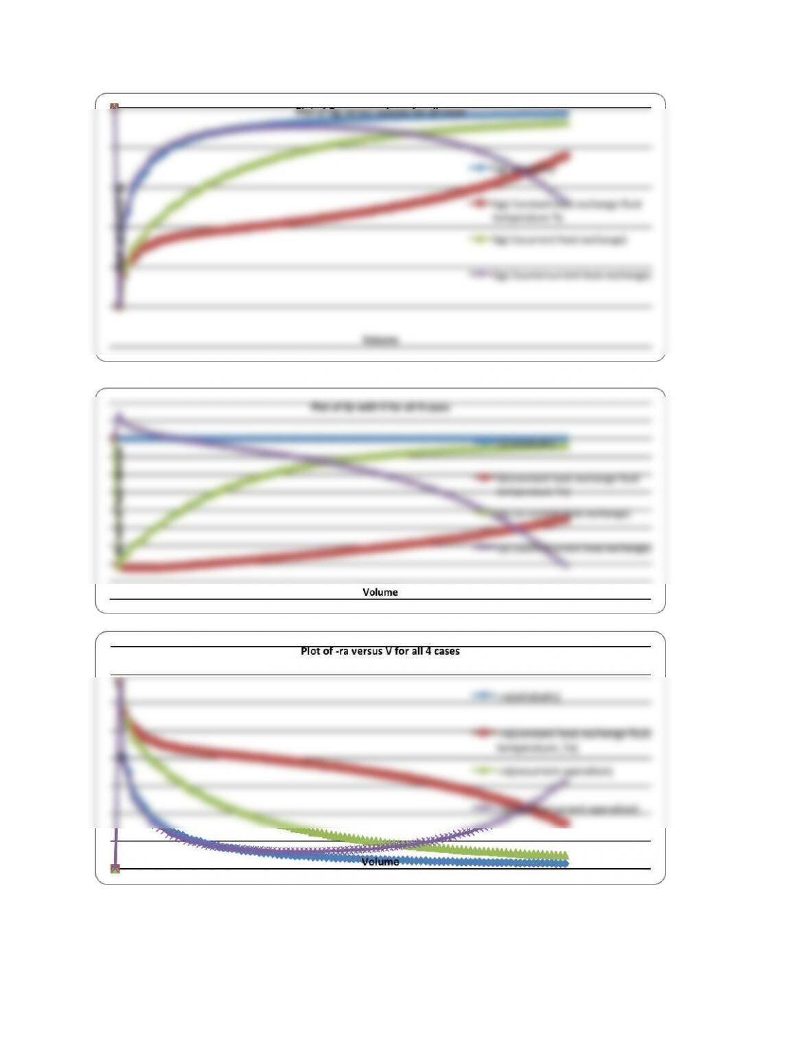
Plot$of$Qr$versus$volume$for$all$cases

$

Plot$of$$–ra$(rate)$versus$V

$

It$can$be$seen$that$the$rate$for$constant$heat$exchange$fluid$temperature$Ta,$is$higher$than$the$rest$of$

cases$because$the$difference$between$heat$generated$and$heat$removed$in$this$case$is$highest.$$

$

12–18$

P12-1)(c))Continued$

The$rate$of$reaction$for$all$cases$is$decreasing$because$the$temperature$of$the$system$is$decreasing$with$

volume.$

(x)$Introduction$of$inert$will$introduce$a$change$in$energy$balance$equation$and$the$value$of$Ѳ1$as$well.$

(xi)$$

(1)$ѲI$=$0$

(2)$ѲI$=$1.5$

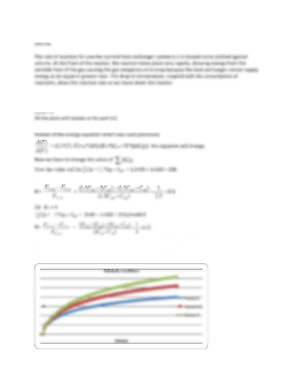
Instead$of$the$energy$equation$which$was$used$previously$$

Value$of$Ѳ$will$change$as$well$

Ѳ$=$

=$

$

$$

$

Incorporating$these$changes$in$the$code$and$plotting$X$versus$V$for$different$cases.$

The$analysis$is$as$follows:$

Case$I:$$adiabatic$operation:$

$

12–19$

P12-1)(c))Continued$

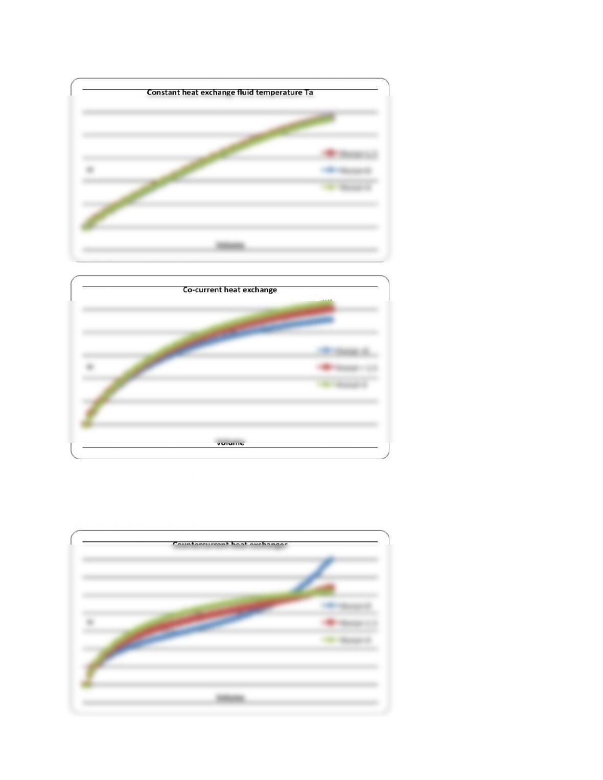
Case2:$Constant$heat$exchange$fluid$temperature$Ta$

$

The$Polymath$program$for$reference$is$for$the$case$of$co–current$heat$exchange$with$ѲI$=3.$

By$changing$values$of$∑Cp$and$ε$variables$as$shown$we$can$change$the$program$for$various$cases$and$

sub$cases.$

Case$4:$$Countercurrent$heat$exchange$

$

12–20$

P12-1)(c))Continued$

Remarks:$Thus$we$can$see$that$for$all$cases$when$inert$gas$concentration$is$more,$then$the$reaction$

proceeds$faster$but$then$the$overall$yield$is$less$as$well.$In$the$case$of$adiabatic$operation$this$

phenomenon$is$very$significant.$In$case$of$constant$heat$exchange$fluid$temperature$the$effect$of$inert$

gas$is$negligible.$

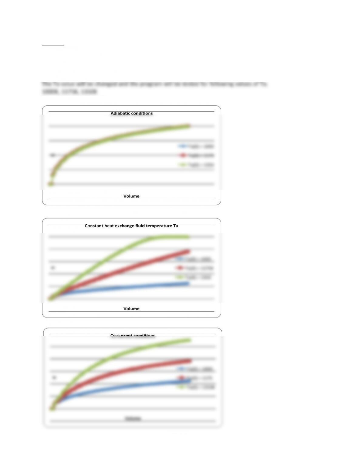
(xii)$Here$we$will$change$the$Polymath$program$as$entered$in$P12–2(c)$part$(vi).$

The$Ta$value$will$be$changed$and$the$program$will$be$tested$for$following$values$of$Ta.$

Case)1:$adiabatic$conditions$

$

Case$2:$Constant$heat$exchange$fluid$temperature$Ta$

$

Case$3:$Co–current$conditions$

$ $