SOLUTION
(10 min.) Absorption and variable costing.
The answers are 1(a) and 2(c). Computations:
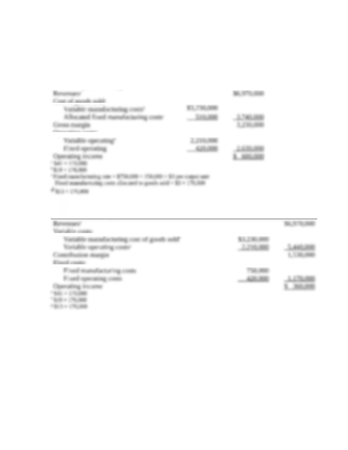
1. Absorption Costing:
Revenuesa
Cost of goods sold:
$6,970,000
Operating costs:
2. Variable Costing:
Revenuese
Variable costs:
Variable manufacturing cost of goods soldf
Variable operating costsg
Contribution margin
Fixed costs:
Fixed manufacturing costs
Fixed operating costs
$3,230,000
2 ,210,000
750,000
420 ,000
$6,970,000
5 ,440,000
1,530,000
1 ,170,000
e $41 × 170,000
f $19 × 170,000
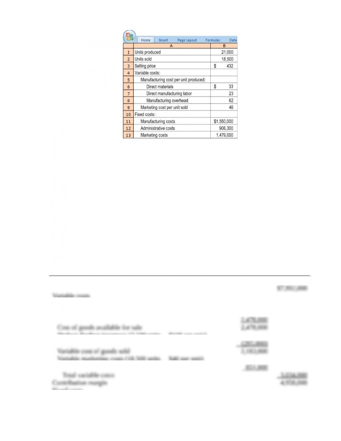
9-27 Absorption versus variable costing. Horace Company manufactures a
professional-grade vacuum cleaner and began operations in 2017. For 2017, Horace budgeted to
produce and sell 25,000 units. The company had no price, spending, or efficiency variances and
writes off production-volume variance to cost of goods sold. Actual data for 2017 are given as
follows:
Required:
1. Prepare a 2017 income statement for Horace Company using variable costing.
2. Prepare a 2017 income statement for Horace Company using absorption costing.
3. Explain the differences in operating incomes obtained in requirements 1 and 2.
4. Horace’s management is considering implementing a bonus for its supervisors based on gross
margin under absorption costing. What incentives will this bonus plan create for the
supervisors? What modifications could Horace management make to improve such a plan?
Explain briefly.
SOLUTION
(40 min) Absorption versus variable costing.
1. The variable manufacturing cost per unit is $33 + $23 + $62 = $118.
2017 Variable-Costing Based Income Statement
Revenues (18,500
´
$432 per unit)
Variable costs
Beginning inventory $ 0
Variable manufacturing costs (21,000 units
´
$118 per unit)
Deduct: Ending inventory (2,500 units
´
$118 per unit)
Variable marketing costs (18,500 units
´
$46 per unit)
Fixed costs
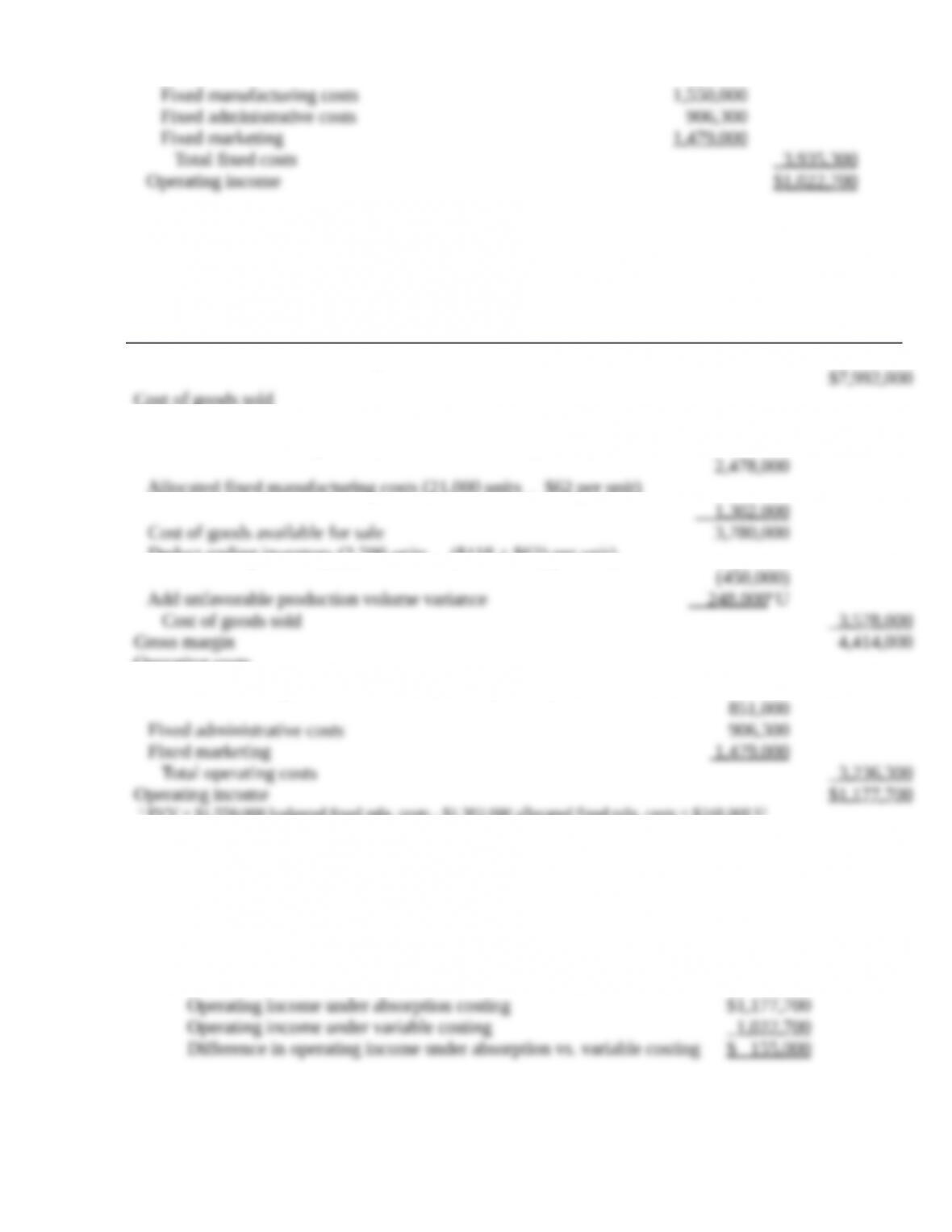
2. Fixed manufacturing overhead rate = $1,550,000 / 25,000 units = $62 per unit
¿$1,100,000 ÷20,000 units=$55 per unit
2017 Absorption-Costing Based Income Statement
Revenues (18,500 units
´
$432 per unit)
Cost of goods sold
Beginning inventory $ 0
Variable manufacturing costs (21,000 units
´
$118 per unit)
Allocated fixed manufacturing costs (21,000 units
´
$62 per unit)
Deduct ending inventory (2,500 units
´
($118 + $62) per unit)
Operating costs
Variable marketing costs (18,500 units
´
$46 per unit)
a PVV = $1,550,000 budgeted fixed mfg. costs – $1,302,000 allocated fixed mfg. costs = $248,000 U
3. 2017 operating income under absorption costing is greater than the operating income
under variable costing because in 2017 inventory increased by 2,500 units. As a result, under
absorption costing, a portion of the fixed overhead remained in the ending inventory, and led to a
lower cost of goods sold (relative to variable costing). As shown below, the difference in the two
operating incomes is exactly the same as the difference in the fixed manufacturing costs included
in ending vs. beginning inventory (under absorption costing).
Under absorption costing:
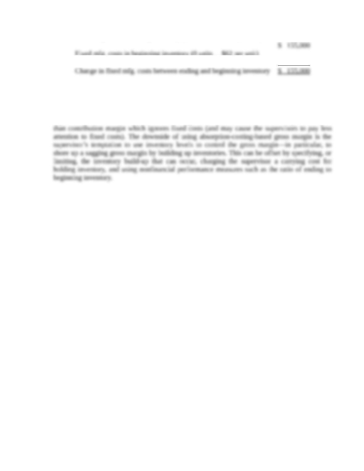
Fixed mfg. costs in ending inventory (2,500 units
´
$62 per unit)
Fixed mfg. costs in beginning inventory (0 units
´
$62 per unit)
0
4. Relative to the alternative of using contribution margin (from variable costing), the
absorption-costing based gross margin has some pros and cons as a performance measure for
Horace’s supervisors. It takes into account both variable costs and fixed costs—costs that the
supervisors should be able to control in the long-run—and therefore is a more complete measure
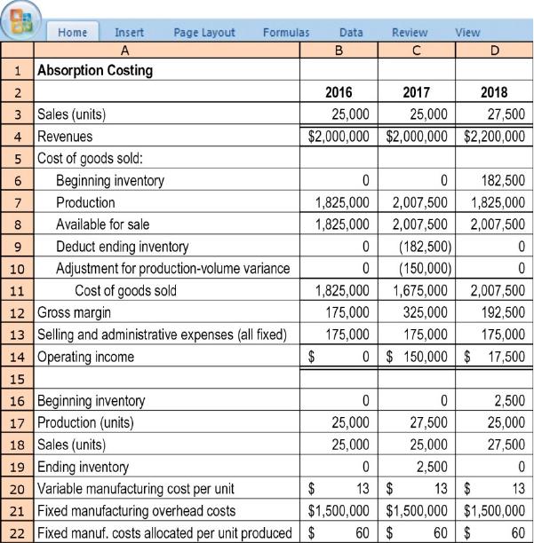
9-28 Variable and absorption costing, sales, and operating-income changes. Candyland
uses standard costing to produce a particularly popular type of candy. Candyland’s president,
Jack McCay, was unhappy after reviewing the income statements for the first three years of
business. He said, “I was told by our accountants—and in fact, I have memorized—that our
breakeven volume is 25,000 units. I was happy that we reached that sales goal in each of our first
two years. But here’s the strange thing: In our first year, we sold 25,000 units and indeed we
broke even. Then in our second year we sold the same volume and had a significant, positive
operating income. I didn’t complain, of course … but here’s the bad part. In our third year, we
sold 10% more candy, but our operating income dropped by nearly 90% from what it was in the
second year! We didn’t change our selling price or cost structure over the past three years and
have no price, efficiency, or spending variances … so what’s going on?!”
Required:
1. What denominator level is Candyland using to allocate fixed manufacturing costs to the
candy? How is Candyland disposing of any favorable or unfavorable production-volume
variance at the end of the year? Explain your answer briefly.
2. How did Candyland’s accountants arrive at the breakeven volume of 25,000 units?
3. Prepare a variable costing-based income statement for each year. Explain the variation in
variable costing operating income for each year based on contribution margin per unit and
sales volume.
4. Reconcile the operating incomes under variable costing and absorption costing for each year,
and use this information to explain to Jack McCay the positive operating income in 2017 and
the drop in operating income in 2018.
SOLUTION
(40 min.) Variable and absorption costing, sales, and operating-income changes.
1. Candyland’s annual fixed manufacturing costs are $1,500,000. It allocates $60 of fixed
manufacturing costs to each unit produced. Therefore, it must be using $1,500,000
¸
$60 =
25,000 units (annually) as the denominator level to allocate fixed manufacturing costs to the
units produced.
We can see from Candyland’s income statements that it disposes of any production volume
variance against cost of goods sold. In 2017, 27,500 units were produced instead of the budgeted
´
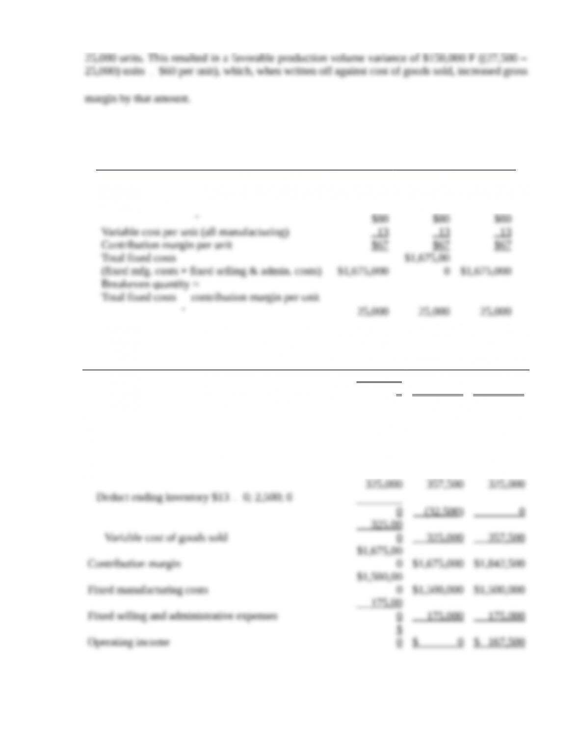
2 The breakeven calculation, same for each year, is shown below:
Calculation of breakeven volume 2016
201
7 2018
Selling price ($2,000,000
¸
25,000; $2,000,000
¸
25,000; $2,200,000
¸
27,500)
¸
3.
Variable Costing
2016 2017 2018
Sales (units)
25,00
0 25,000 27,500
Revenues
$2,000,00
0 $2,000,000 $2,200,000
Variable cost of goods sold
Beginning inventory $13
´
0; 0; 2,500
0 0 32,500
Variable manuf. costs $13
´
25,000; 27,500; 25,000
´
Explaining variable costing operating income
Contribution margin
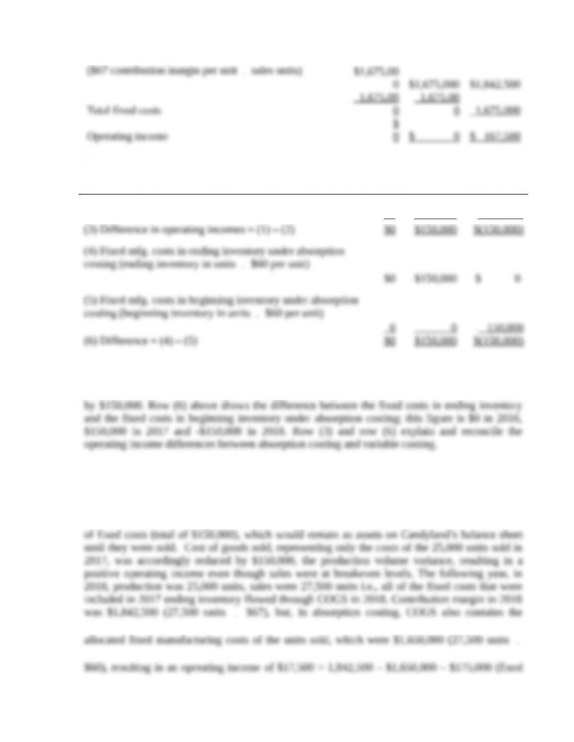
4.
Reconciliation of absorption/variable costing
operating incomes 2016 2017 2018
(1) Absorption costing operating income $0 $150,000 $ 17,500
(2) Variable costing operating income 0 0 167 ,500
´
´
In the table above, row (3) shows the difference between the operating income under absorption
costing and the operating income under variable costing, for each of the three years. In 2016, the
difference is $0; in 2017, absorption costing income is greater by $150,000; and in 2018, it is less
Jack McCay is surprised at the non-zero, positive net income (reported under absorption
costing) in 2017, when sales were at the ‘breakeven volume’ of 25,000; further, he is concerned
about the drop in operating income in 2018, when, in fact, sales increased to 27,500 units. In
2017, starting with zero inventories, 27,500 units were produced and 25,000 were sold, i.e., at
the end of the year, 2,500 units remained in inventory. These 2,500 units had each absorbed $60
´
´
sales and admin.) Hence the drop in operating income under absorption costing, even though
sales were greater than the computed breakeven volume: inventory levels decreased sufficiently
Note that beginning and ending with zero inventories during the 2016-2018 period, under
both costing methods, Candyland’s total operating income was $167,500.
9-29 Capacity management, denominator-level capacity concepts.
Match each of the following numbered descriptions with one or more of the denominator-level
capacity concepts by putting the appropriate letter(s) by each item:
a. Theoretical capacity
b. Practical capacity
c. Normal capacity utilization
d. Master-budget capacity utilization
1. Measures the denominator level in terms of what a plant can supply
2. Is based on producing at full efficiency all the time
3. Represents the expected level of capacity utilization for the next budget period
4. Measures the denominator level in terms of demand for the output of the plant
5. Takes into account seasonal, cyclical, and trend factors
6. Should be used for performance evaluation in the current year
7. Represents an ideal benchmark
8. Highlights the cost of capacity acquired but not used
9. Should be used for long-term pricing purposes
10. Hides the cost of capacity acquired but not used
11. If used as the denominator-level concept, would avoid the restatement of unit costs when
expected demand levels change
SOLUTION
(10 min.) Capacity management, denominator-level capacity concepts.
1. a, b
2. a
3. d
9-30 Denominator-level problem. Thunder Bolt, Inc., is a manufacturer of the very
popular G36 motorcycles. The management at Thunder Bolt has recently adopted absorption
costing and is debating which denominator-level concept to use. The G36 motorcycles sell for an
average price of $8,200. Budgeted fixed manufacturing overhead costs for 2017 are estimated at
$6,480,000. Thunder Bolt, Inc., uses subassembly operators that provide component parts. The
following are the denominator-level options that management has been considering:
a. Theoretical capacity—based on three shifts, completion of five motorcycles per shift, and a
360-day year —3 5 360 = 5,400.
b. Practical capacity—theoretical capacity adjusted for unavoidable interruptions, breakdowns,
and so forth —3 4 320 = 3,840.
c. Normal capacity utilization—estimated at 3,240 units.
d. Master-budget capacity utilization—the strengthening stock market and the growing
popularity of motorcycles have prompted the marketing department to issue an estimate for
2017 of 3,600 units.
Required:
1. Calculate the budgeted fixed manufacturing overhead cost rates under the four denominator-level
concepts.
2. What are the benefits to Thunder Bolt, Inc., of using either theoretical capacity or practical
capacity?
3. Under a cost-based pricing system, what are the negative aspects of a master-budget
denominator level? What are the positive aspects?
SOLUTION
(20 min.) Denominator-level problem.
1. Budgeted fixed manufacturing overhead costs rates:
Denominator
Level Capacity
Concept
Budgeted Fixed
Manufacturing
Overhead per
Period
Budgeted
Capacity
Level
Budgeted Fixed
Manufacturing
Overhead Cost
Rate
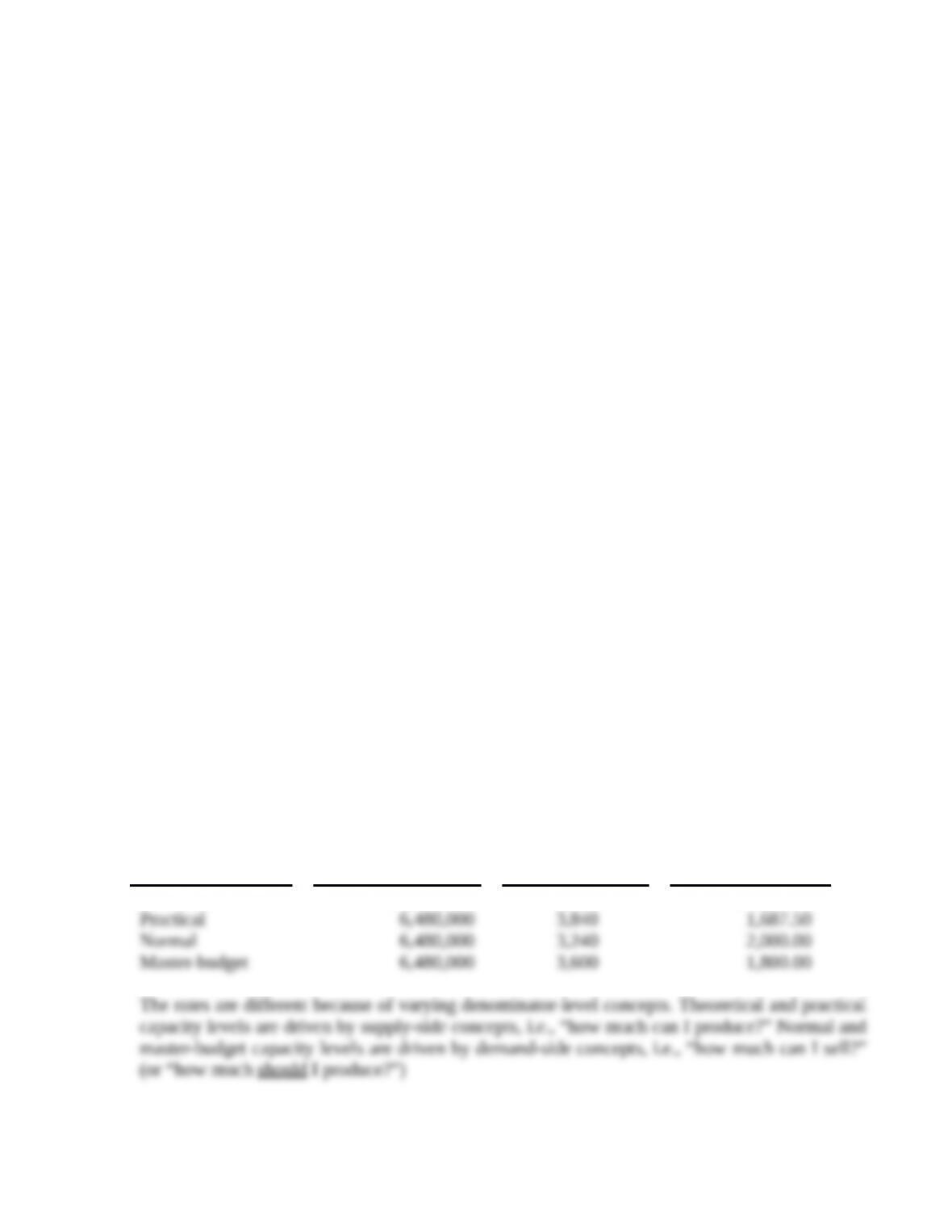
Theoretical $ 6,480,000 5,400 $ 1,200.00
2. The variances that arise from use of the theoretical or practical level concepts will signal
that there is a divergence between the supply of capacity and the demand for capacity. This is
3. Under a cost-based pricing system, the choice of a master-budget level denominator will
lead to high prices when demand is low (more fixed costs allocated to the individual product
level), further eroding demand; conversely, it will lead to low prices when demand is high,
9-31 Variable and absorption costing and breakeven points. Camino, a leading firm in the
sports industry, produces basketballs for the consumer market. For the year ended December 31,
2017, Camino sold 400,000 basketballs at an average selling price of $12 per unit. The following
information also relates to 2017 (assume constant unit costs and no variances of any kind):
Inventory, January 1, 2017: 0 basketballs
Inventory, December 31, 2017: 20,000 basketballs
Fixed manufacturing costs: $380,000
Fixed administrative costs: $660,000
Direct materials costs: $ 3 per basketball
Direct labor costs: $ 4 per basketball
Required:
1. Calculate the breakeven point (in basketballs sold) in 2017 under:
a. Variable costing
b. Absorption costing
2. Suppose direct materials costs were $4 per basketball instead. Assuming all other data are the
same, calculate the minimum number of basketballs Camino must have sold in 2017 to attain
a target operating income of $120,000 under:
a. Variable costing
b. Absorption costing
SOLUTION
(30 min.)Variable and absorption costing and breakeven points.
1. Production = Sales + Ending Inventory – Beginning Inventory

= 400,000 + 0 20,000
= 380,000 basketballs.
Breakeven point in units (basketballs sold):
a. Variable Costing:
Q=
Per UnitMargin on Contributi
Income OperatingTarget Costs Fixed Total
Q=
($380,000 $660,000) $0
$12 – $3 – $4
+ +
Q=
$1,040,000
$5
Q = 208,000 units.
b. Absorption costing:
Fixed manufacturing cost rate = $380,000 ÷ 380,000 = $1 per unit
Q =
( )
Total Fixed Target Fixed Manuf. Breakeven Units
Cost OI Cost Rate Sales in Units Produced
Contribution Margin Per Unit
é ù
+ + ´ –
ê ú
ë û
Q =
[ ]
$1,040,000 $0 $1 (Q 380,000)
$5
+ + –
Q =
$1,040,000 Q $380,000
$5
+ –
Q =
$660,000 Q
$5
+
4 Q = $660,000
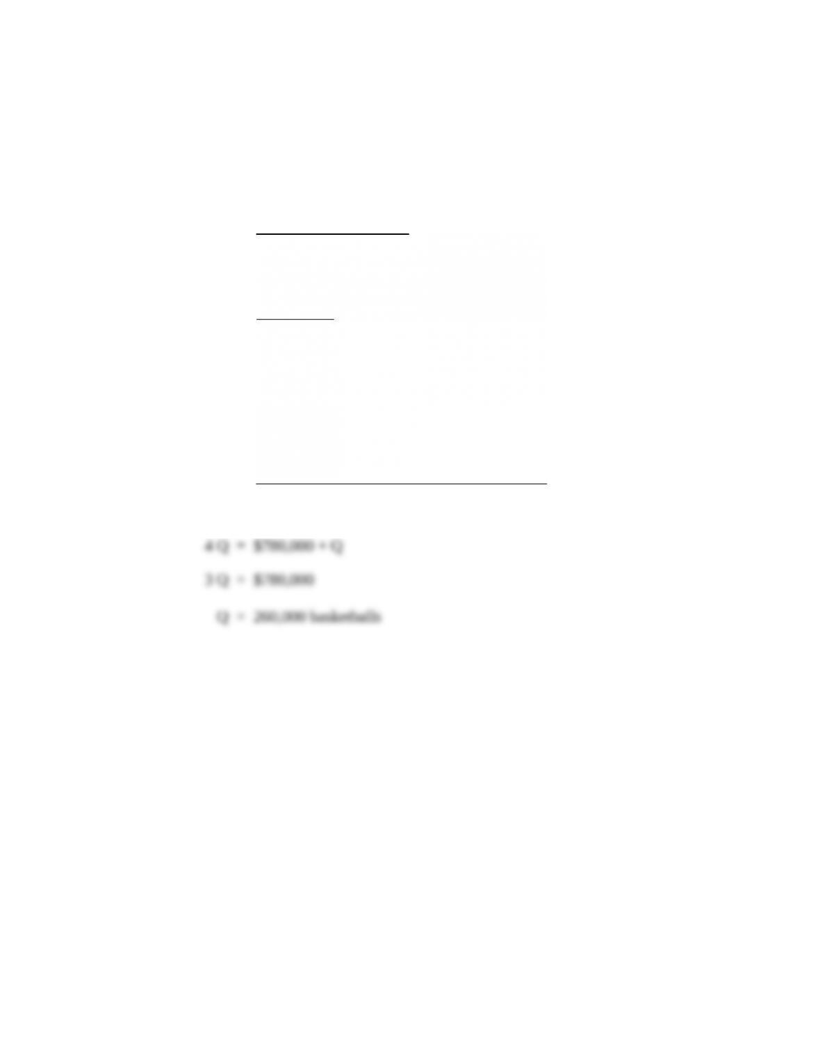
Q = 165,000 basketballs.
2. If direct materials costs were $4 instead per basketball, the contribution margin would be
lowered to $4.
a. Variable Costing:
Q =
$1,040,000 $120,000
$4
+
=
$1,160,000
$4
= 290,000 basketballs
b. Absorption Costing:
Q =
[ ]
$1,040,000 $120,000 $1 (Q 380,000)
$4
+ + –
9-32 Variable costing versus absorption costing. The Garvis Company uses
an absorption-costing system based on standard costs. Variable manufacturing cost consists of
direct material cost of $4.50 per unit and other variable manufacturing costs of $1.50 per unit.
The standard production rate is 20 units per machine-hour. Total budgeted and actual fixed
manufacturing overhead costs are $840,000. Fixed manufacturing overhead is allocated at $14
per machine-hour based on fixed manufacturing costs of [&~univers57~\$840,000|div|60,000&]
machine-hours, which is the level Garvis uses as its denominator level.
The selling price is $10 per unit. Variable operating (nonmanufacturing) cost, which is driven
by units sold, is $2 per unit. Fixed operating (nonmanufacturing) costs are $240,000. Beginning
inventory in 2017 is 60,000 units; ending inventory is 80,000 units. Sales in 2017 are 1,080,000
units.
The same standard unit costs persisted throughout 2016 and 2017. For simplicity, assume that
there are no price, spending, or efficiency variances.
Required:
1. Prepare an income statement for 2017 assuming that the production-volume variance is
written off at year-end as an adjustment to cost of goods sold.
2. The president has heard about variable costing. She asks you to recast the 2017 statement as
it would appear under variable costing.
3. Explain the difference in operating income as calculated in requirements 1 and 2.
4. Graph how fixed manufacturing overhead is accounted for under absorption costing. That is,
there will be two lines: one for the budgeted fixed manufacturing overhead (which is equal to
the actual fixed manufacturing overhead in this case) and one for the fixed manufacturing
overhead allocated. Show the production-volume variance in the graph.
5. Critics have claimed that a widely used accounting system has led to undesirable buildups of
inventory levels. (a) Is variable costing or absorption costing more likely to lead to such
buildups? Why? (b) What can managers do to counteract undesirable inventory buildups?