SOLUTION
(25–30 min.) Flexible-budget preparation and analysis.
1. Variance Analysis for Bank Management Printers for September 2017
Level 1 Analysis
Actual
Results
(1)
Static-Budget
Variances
(2) = (1) – (3)
Static
Budget
(3)
Units sold
12 ,000
3 ,000 U
15 ,000
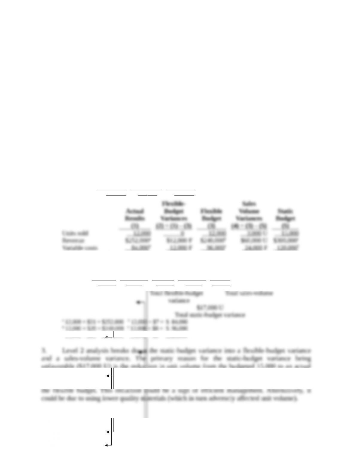
2. Level 2 Analysis
Actual
Results
(1)
Flexible-
Budget
Variances
(2) = (1) – (3)
Flexible
Budget
(3)
Sales
Volume
Variances
(4) = (3) – (5)
Static
Budget
(5)
Units sold 12 ,000 0 12 ,000 3 ,000 U 15 ,000
Revenue $252,000a$12,000 F $240,000b$60,000 U $300,000c
Total flexible-budget Total sales-volume
variance
3. Level 2 analysis breaks down the static-budget variance into a flexible-budget variance
and a sales-volume variance. The primary reason for the static-budget variance being
unfavorable ($17,000 U) is the reduction in unit volume from the budgeted 15,000 to an actual
7-1
7-24 Flexible budget, working backward. The Clarkson Company produces engine parts for
car manufacturers. A new accountant intern at Clarkson has accidentally deleted the company’s vari–
ance analysis calculations for the year ended December 31, 2017. The following table is what re–
mains of the data.
Required:
1. Calculate all the required variances. (If your work is accurate, you will find that the total stat–
ic-budget variance is $0.)
2. What are the actual and budgeted selling prices? What are the actual and budgeted variable costs
per unit?
3. Review the variances you have calculated and discuss possible causes and potential prob–
lems. What is the important lesson learned here?
SOLUTION
(30 min.) Flexible budget, working backward.
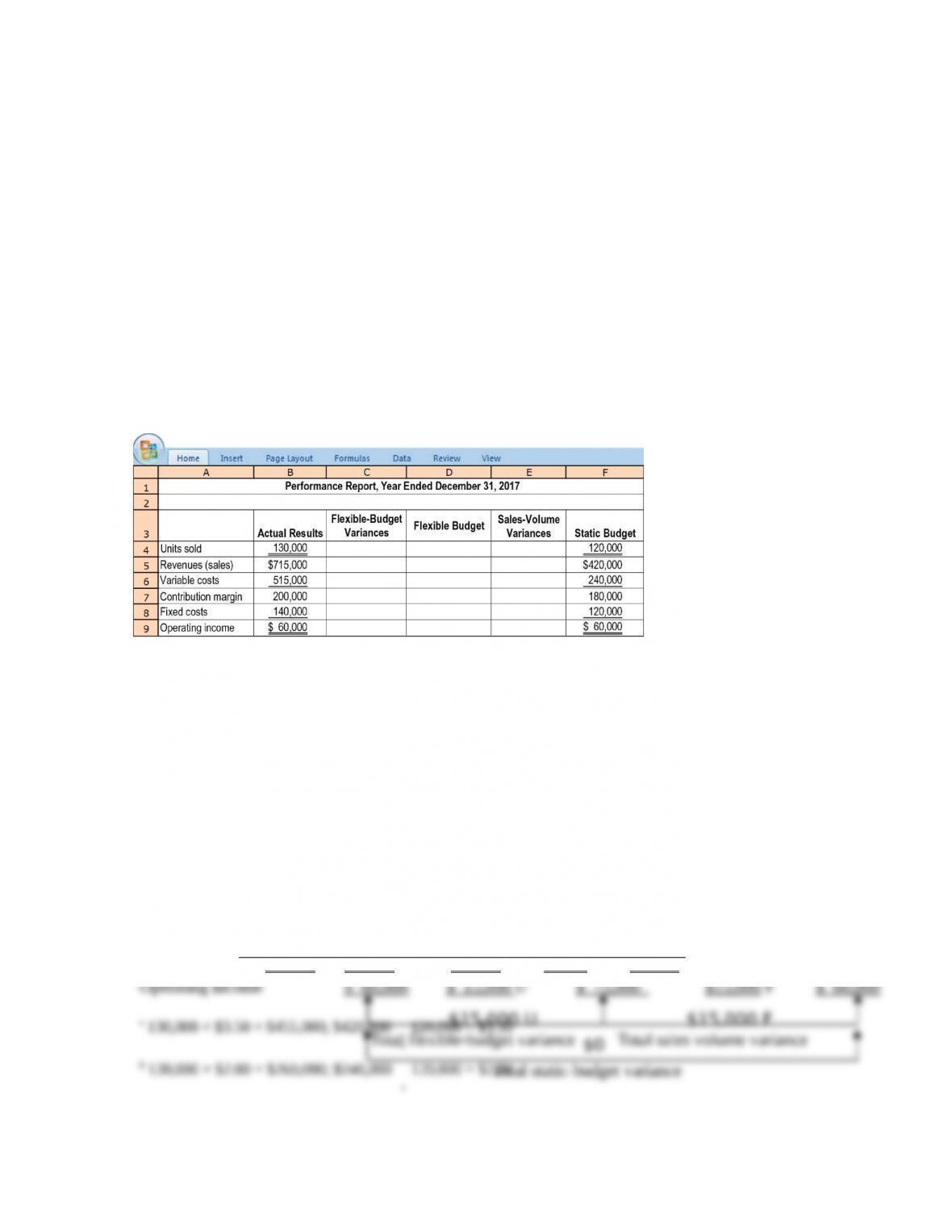
1. Variance Analysis for The Clarkson Company for the year ended December 31, 2017
Actual
Results
(1)
Flexible-
Budget
Variances
(2)=(1)(3)
Flexible
Budget
(3)
Sales-Volume
Variances
(4)=(3)(5)
Static
Budget
(5)
Units sold 130,000 0 130 ,000 10 ,000 F 120,000
Revenues $715,000 $260,000 F $455,000a$35,000 F $420,000
b 130,000 × $2.00 = $260,000; $240,000
¸
7-2
$0
¸
2. Actual selling price: $715,000
Budgeted selling price: 420,000
Actual variable cost per unit: 515,000
3. A zero total static-budget variance may be due to offsetting total flexible-budget and total
sales-volume variances. In this case, these two variances exactly offset each other:
Total flexible-budget variance $15,000 Unfavorable
Total sales-volume variance $15,000 Favorable
A closer look at the variance components reveals some major deviations from plan.
Actual variable costs increased from $2.00 to $3.96, causing an unfavorable flexible-budget
variable cost variance of $255,000. Such an increase could be a result of, for example, a jump in
direct material prices. Clarkson was able to pass most of the increase in costs onto their
customers—actual selling price increased by 57% [($5.50 – $3.50)
¸
$3.50], bringing about an
7-3
7-25 Flexible-budget and sales volume variances. Cascade, Inc., produces the basic fillings used in many popular
frozen desserts and treats—vanilla and chocolate ice creams, puddings, meringues, and fudge. Cascade uses standard costing and carries
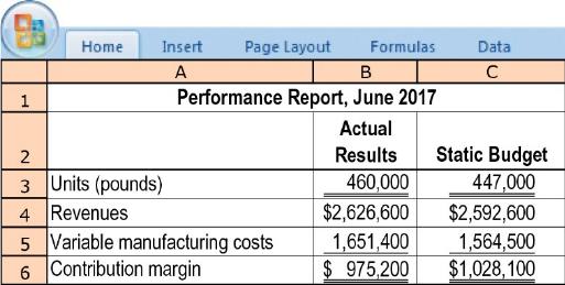
over no inventory from one month to the next. The ice-cream product group’s results for June 2017 were as follows:
Jeff Geller, the business manager for ice-cream products, is pleased that more pounds of ice cream were sold than budgeted and that rev–
enues were up. Unfortunately, variable manufacturing costs went up, too. The bottom line is that contribution margin declined by $52,900,
which is just over 2% of the budgeted revenues of $2,592,600. Overall, Geller feels that the business is running fine.
Required:
1. Calculate the static-budget variance in units, revenues, variable manufacturing costs, and contribution margin. What percentage
is each static-budget variance relative to its static-budget amount?
2. Break down each static-budget variance into a flexible-budget variance and a sales-volume variance.
3. Calculate the selling-price variance.
4. Assume the role of management accountant at Cascade. How would you present the results to Jeff Geller? Should he be more con–
cerned? If so, why?
SOLUTION
(30-40 min.) Flexible budget and sales volume variances, market-share and market-size variances.
1. and 2.
7-4
Performance Report for Cascade, Inc., June 2017
Actual
Flexible
Budget
Variances
Flexible
Budget
Sales Volume
Variances
Static
Budget
Static
Budget
Variance
Static Budget
Variance as
% of Static
Budget
(1) (2) = (1) – (3) (3) (4) = (3) – (5) (5) (6) = (1) – (5)
(7) = (6)
¸
(5)
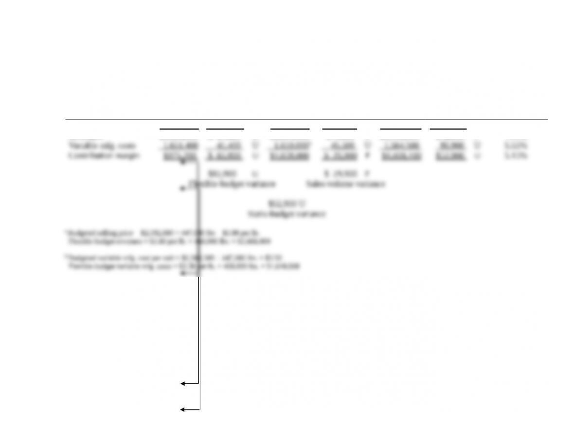
Units (pounds) 460,000 – 460,000 13,000 F 447,000 13,000 F 2.91%
Revenues $2,626,600 $ 41,400 U $2,668,000a $75,400 F $2,592,600 $34,000 F 1.31%
7-5

3. The selling price variance, caused solely by the difference in actual and budgeted selling
4. The flexible-budget variances show that for the actual sales volume of 460,000 pounds,
selling prices were lower and costs per pound were higher. The favorable sales volume variance
in revenues (because more pounds of ice cream were sold than budgeted) helped offset the
7-26 Price and efficiency variances. Sunshine Foods manufactures pumpkin scones. For Jan–
uary 2017, it budgeted to purchase and use 14,750 pounds of pumpkin at $0.92 a pound. Actual
purchases and usage for January 2017 were 16,000 pounds at $0.85 a pound. Sunshine budgeted
for 59,000 pumpkin scones. Actual output was 59,200 pumpkin scones.
Required:
1. Compute the flexible-budget variance.
2. Compute the price and efficiency variances.
3. Comment on the results for requirements 1 and 2 and provide a possible explanation for
them.
SOLUTION
(20–30 min.) Price and efficiency variances.
1. The key information items are:
Actual Budgeted
Output units (scones)
59,200
59,000
Actual
Results
(1)
Flexible-
Budget
Variance
(2) = (1) – (3)
Flexible
Budget
(3)
Sales-Volume
Variance
(4) = (3) – (5)
Static
Budget
(5)
Pumpkin costs $13,600a$16 F $13,616b$46 U $13,570c
c 59,000 × 0.25 × $0.92 = $13,570
2.
Actual Costs
Incurred
(Actual Input Qty.
× Actual Price)
Actual Input Qty.
× Budgeted Price
Flexible Budget
(Budgeted Input
Qty. Allowed for
Actual Output
× Budgeted Price)
$13,600a$14,720b$13,616c
$1,120 F $1,104 U
Price variance Efficiency variance
$16 F
Flexible-budget variance
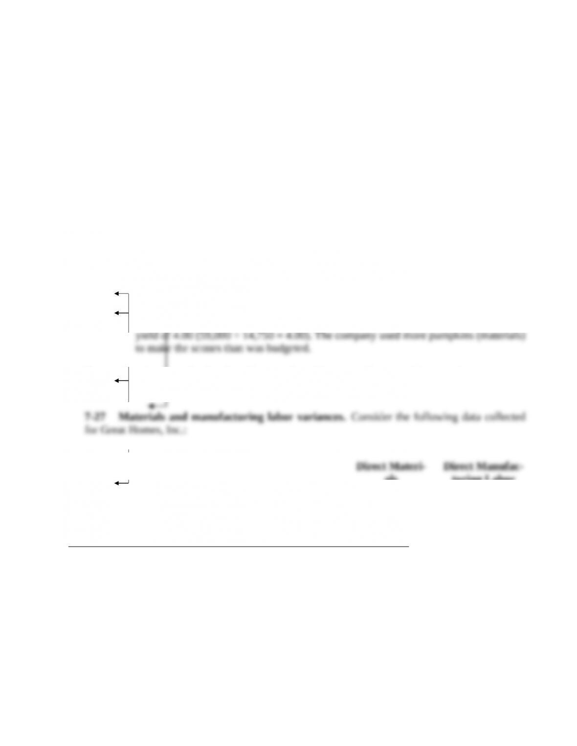
3. The favorable flexible-budget variance of $16 has two offsetting components:
(a) favorable price variance of $1,120––reflects the $0.85 actual purchase cost being
lower than the $0.92 budgeted purchase cost per pound.
7-27 Materials and manufacturing labor variances. Consider the following data collected
for Great Homes, Inc.:
Direct Materi-
als
Direct Manufac-
turing Labor
Cost incurred: Actual inputs actual prices $200,000 $90,000
Actual inputs standard prices 214,000 86,000
Standard inputs allowed for actual output standard
prices
225,000 80,000
Required:
Compute the price, efficiency, and flexible-budget variances for direct materials and direct manufac-
turing labor.
SOLUTION
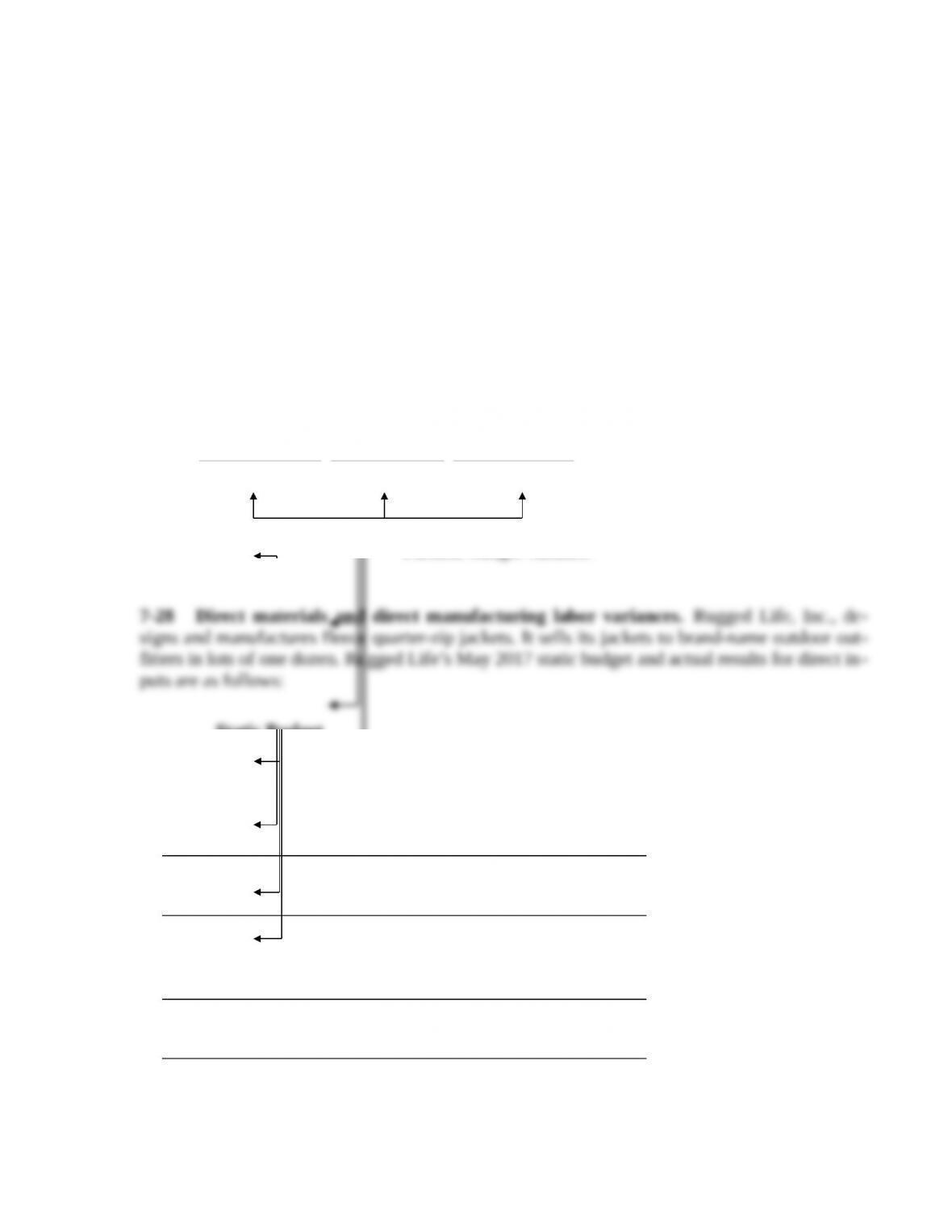
(15 min.) Materials and manufacturing labor variances.
Actual Costs
Incurred
(Actual Input Qty.
× Actual Price)
Actual Input Qty.
× Budgeted Price
Flexible Budget
(Budgeted Input
Qty. Allowed for
Actual Output
× Budgeted Price)
Direct
Materials
$200,000 $214,000 $225,000
$14,000 F $11,000 F
Price variance Efficiency variance
7-28 Direct materials and direct manufacturing labor variances. Rugged Life, Inc., de-
signs and manufactures fleece quarter-zip jackets. It sells its jackets to brand-name outdoor out–
fitters in lots of one dozen. Rugged Life’s May 2017 static budget and actual results for direct in–
puts are as follows:
Static Budget
Number of jacket lots (1 lot = 1 dozen) 300
Per Lot of Jackets:
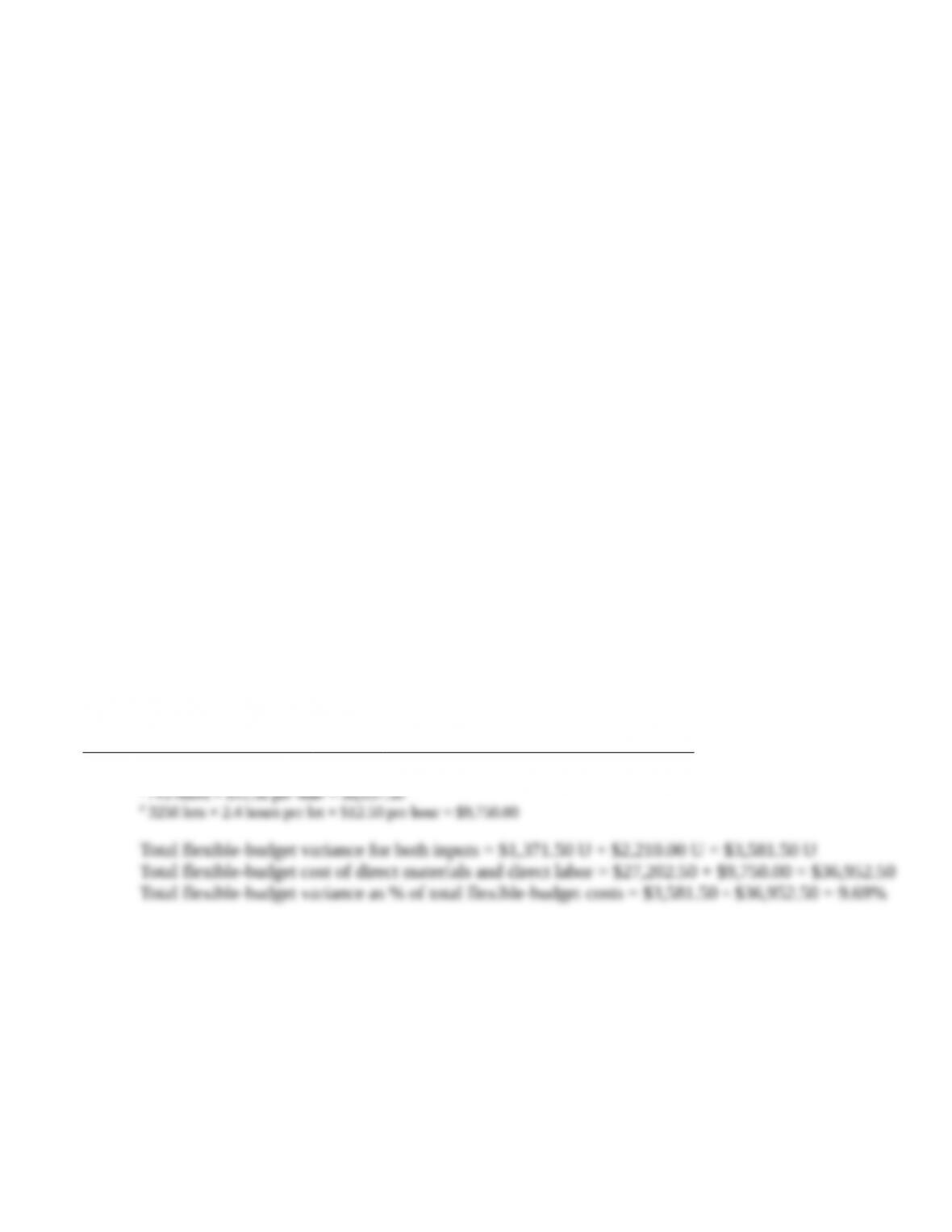
Direct materials 18 yards at $4.65 per yard = $83.70
Direct manufacturing labor 2.4 hours at $12.50 per hour = $30.00
Actual Results
Number of jacket lots sold 325
Total Direct Inputs:
Direct materials 6,500 yards at $4.85 per yard = $31,525
Direct manufacturing labor 715 hours at $12.60 = $9,009
Rugged Life has a policy of analyzing all input variances when they add up to more than 8% of the
total cost of materials and labor in the flexible budget, and this is true in May 2017. The production
manager discusses the sources of the variances: “A new type of material was purchased in May.
This led to faster cutting and sewing, but the workers used more material than usual as they learned
to work with it. For now, the standards are fine.”
Required:
1. Calculate the direct materials and direct manufacturing labor price and efficiency variances
in May 2017. What is the total flexible-budget variance for both inputs (direct materials and
direct manufacturing labor) combined? What percentage is this variance of the total cost of
direct materials and direct manufacturing labor in the flexible budget?
2. Comment on the May 2017 results. Would you continue the “experiment” of using the new
material?
SOLUTION
(20 min.) Direct materials and direct manufacturing labor variances.
1.
May 2017
Actual
Results
Price
Variance
Actual
Quantity
´
Budgeted
Price
Efficiency
Variance
Flexible
Budget
(1) (2) = (1)–(3) (3) (4) = (3) – (5) (5)
Lots 325 325
Direct materials $31,525.00 $1,300.00 U $30,225.00a
$3,022.5
0 U $27,202.50b
2. It is unclear whether the excess use of materials will continue, or whether it was indeed
a result of workers getting accustomed to the new fabric. The time required was indeed lower as
predicted, but not nearly enough to overcome the unfavorable direct material efficiency variance.
7-29 Price and efficiency variances, journal entries. The Schuyler Corporation manufac-
tures lamps. It has set up the following standards per finished unit for direct materials and direct
manufacturing labor:
Direct materials: 10 lb. at $4.50 per lb. $45.00
Direct manufacturing labor: 0.5 hour at $30 per hour 15.00
The number of finished units budgeted for January 2017 was 10,000; 9,850 units were actually
produced.
Actual results in January 2017 were as follows:
Direct materials: 98,055 lb. used
Direct manufacturing labor: 4,900 hours $154,350
Assume that there was no beginning inventory of either direct materials or finished units.
During the month, materials purchased amounted to 100,000 lb., at a total cost of $465,000.
Input price variances are isolated upon purchase. Input-efficiency variances are isolated at the
time of usage.
Required:
1. Compute the January 2017 price and efficiency variances of direct materials and direct manufac-
turing labor.
2. Prepare journal entries to record the variances in requirement 1.
3. Comment on the January 2017 price and efficiency variances of Schuyler Corporation.
4. Why might Schuyler calculate direct materials price variances and direct materials efficiency
variances with reference to different points in time?