SOLUTION
(30–40 min.) Cost estimation, cumulative average-time learning curve.
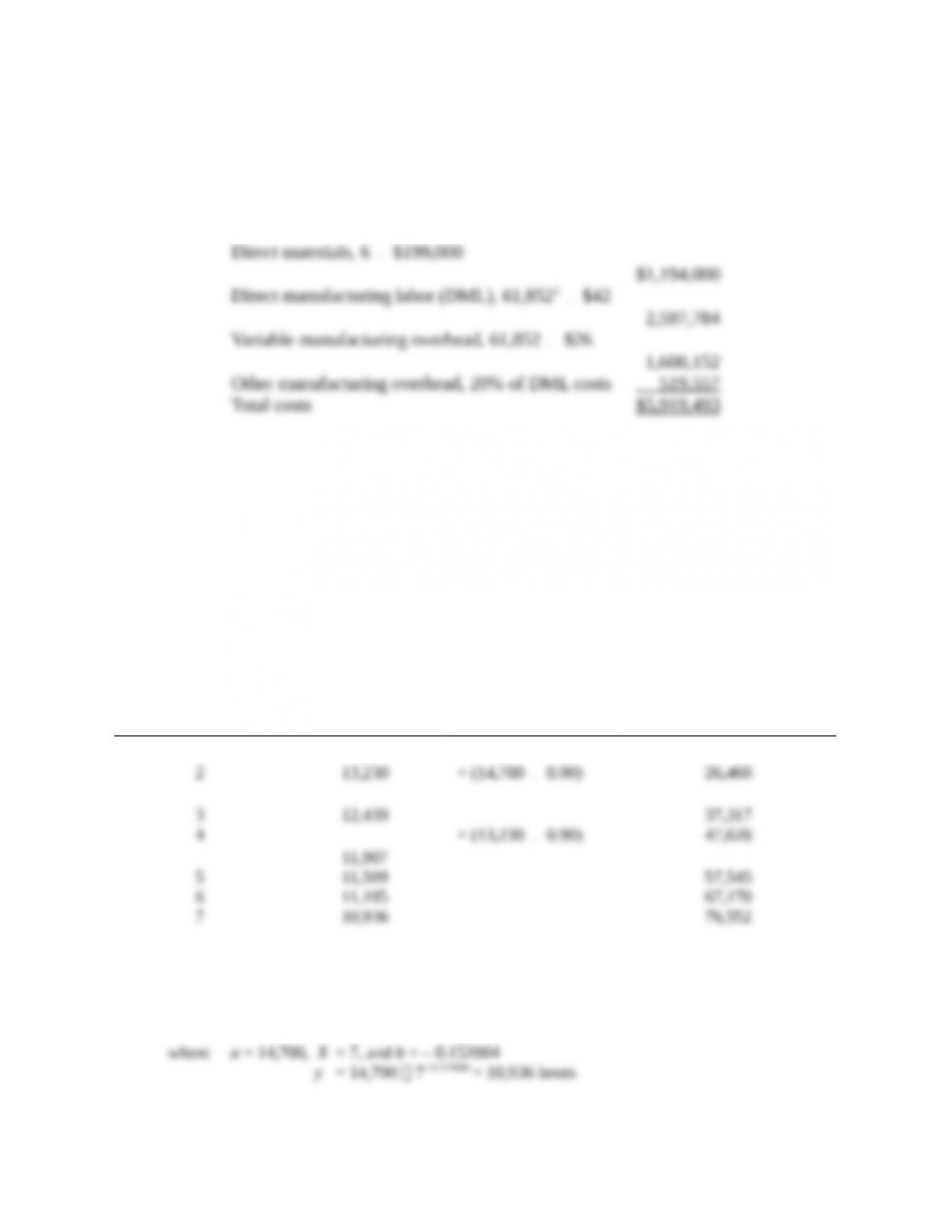
1. Cost to produce the 2nd through the 7th troop deployment boats:
´
´
´
1The direct manufacturing labor-hours to produce the second to seventh boats can be calculated in several
ways, given the assumption of a cumulative average-time learning curve of 90%:
Use of table format:
Cumulative
Number of Units (X)
(1)
90% Learning Curve
Cumulative
Average Time per Unit (y): Labor Hours
(2)
Cumulative
Total Time:
Labor-Hours
(3) = (1)
´
(2)
1 14,700 14,700
´
´
The direct labor-hours required to produce the second through the seventh boats is 76,552 – 14,700 =
61,852 hours.
Use of formula: y = aXb
10-1
The total direct labor-hours for 7 units is 10,936 7 = 76,552 hours
Note: Some students will debate the exclusion of the $279,000 tooling cost. The question
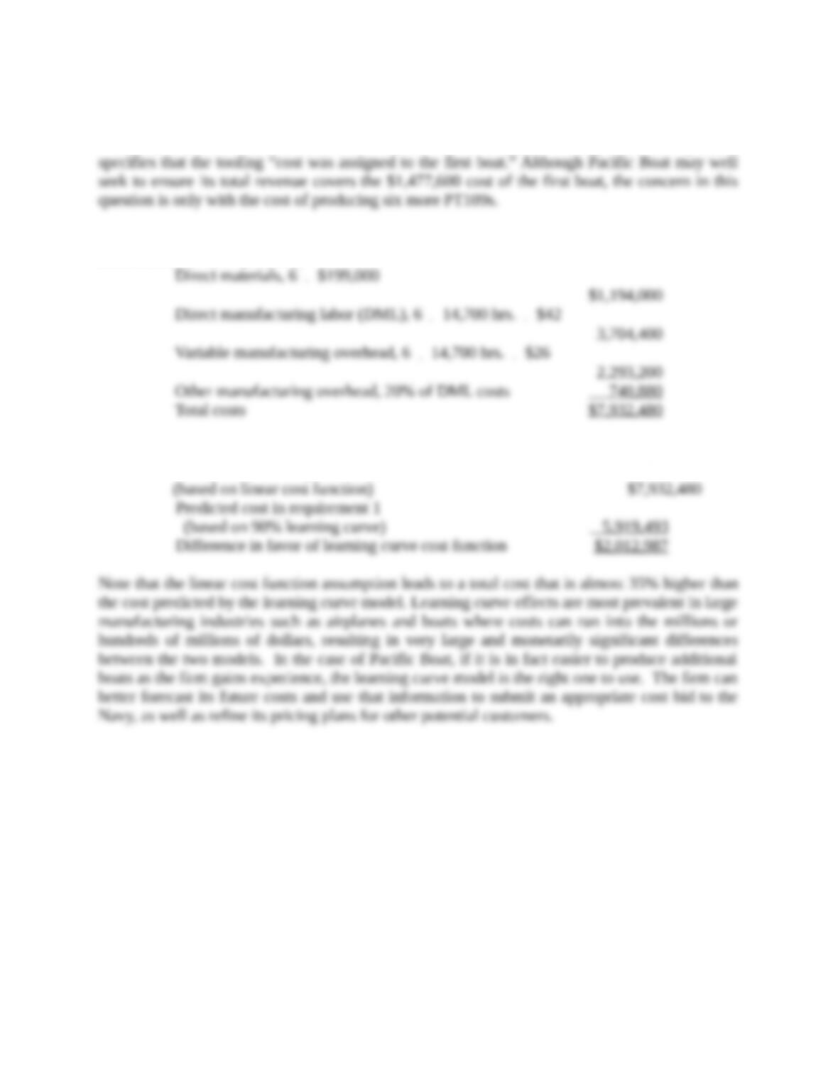
2. Cost to produce the 2nd through the 7th boats assuming linear function for direct
labor-hours and units produced:
The difference in predicted costs is:
Predicted cost in requirement 2
10-41 Cost estimation, incremental unit-time learning model. Assume
the same information for the Pacific Boat Company as in Problem 10-40 with one exception.
This exception is that Pacific Boat uses a 90% incremental unit-time learning model as a basis
for predicting direct manufacturing labor-hours in its assembling operations. (A 90% learning
curve means
b = –0.152004.)
Required:
1. Prepare a prediction of the total costs for producing the six PT109s for the Navy.
2. If you solved requirement 1 of Problem 10-40, compare your cost prediction there with the
one you made here. Why are the predictions different? How should Pacific Boat decide
which model it should use?
10-2
SOLUTION
(20–30 min.) Cost estimation, incremental unit-time learning model.
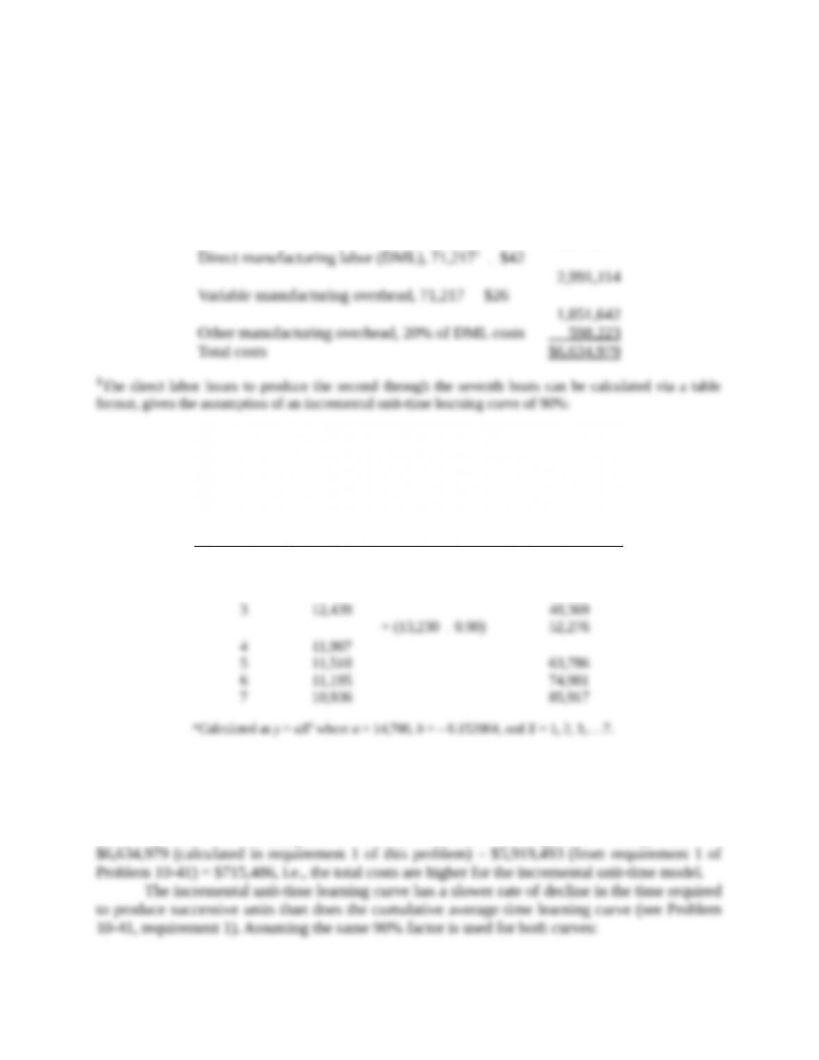
1. Cost to produce the 2nd through the 7th boats:
Direct materials, 6
´
$199,000
$1,194,000
´
´
90% Learning Curve
Cumulative
Number of
Units (X)
Individual Unit Time for Xth
Unit (y)*: Labor Hours
Cumulative
Total Time:
Labor-Hours
(1) (2) (3)
1 14,700 14,700
2
13,230 = (14,700
´
0.90) 27,930
The direct manufacturing labor-hours to produce the second through the seventh boat is 85,917 –
14,700 = 71,217 hours.
2. Difference in total costs to manufacture the second through the seventh boat under the
incremental unit-time learning model and the cumulative average-time learning model is
10-3
Estimated Cumulative Direct Manufacturing Labor-Hours
Cumulative
Number of Units
Cumulative Average-
Time Learning Model
Incremental Unit-Time
Learning Model
1
14,700
14,700
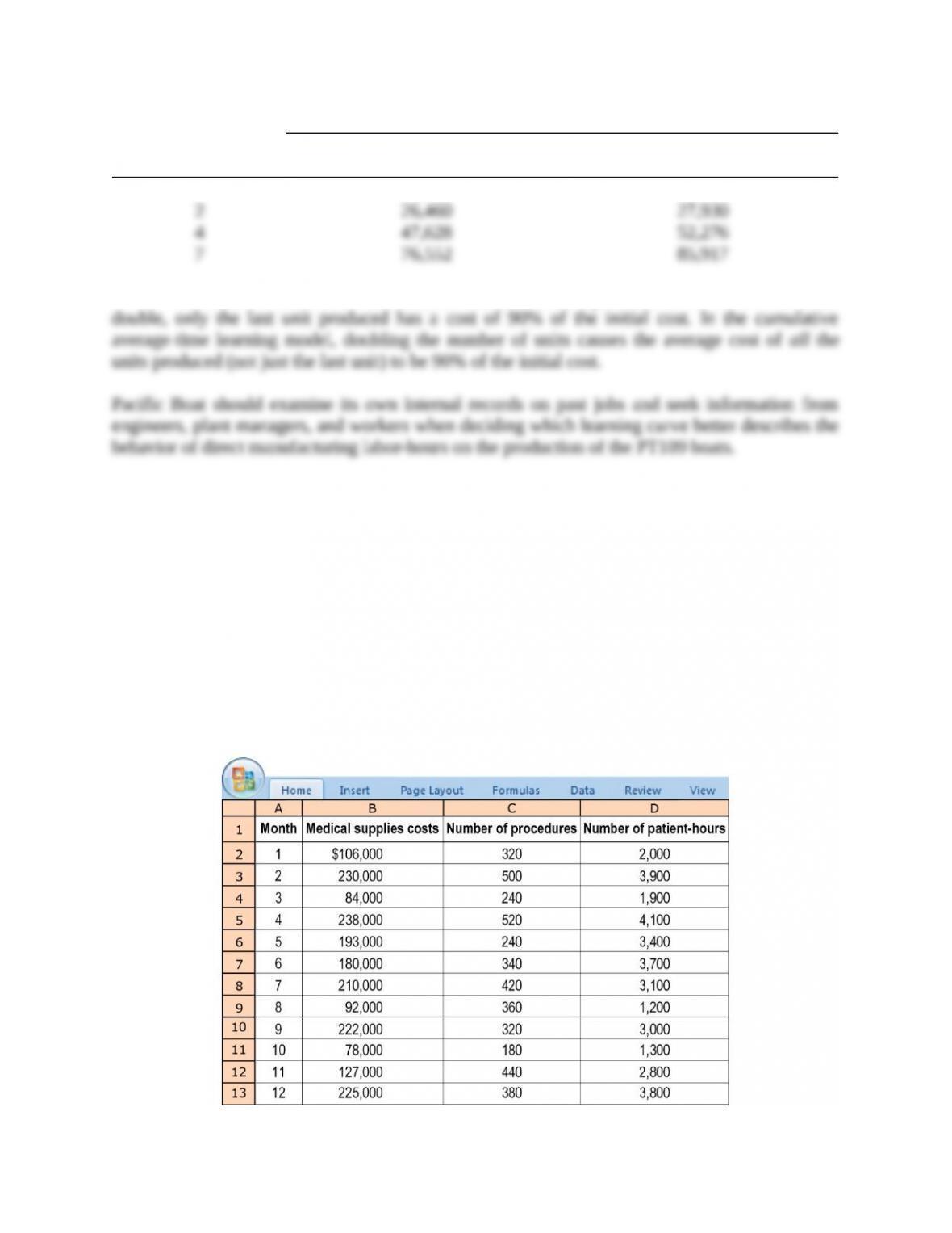
The reason is that, in the incremental unit-time learning model, as the number of units
10-42 Regression; choosing among models. Apollo Hospital specializes in outpatient
surgeries for relatively minor procedures. Apollo is a nonprofit institution and places great
emphasis on controlling costs in order to provide services to the community in an efficient
manner.
Apollo’s CFO, Julie Chen, has been concerned of late about the hospital’s consumption of
medical supplies. To better understand the behavior of this cost, Julie consults with Rhett Bratt,
the person responsible for Apollo’s cost system. After some discussion, Julie and Rhett conclude
that there are two potential cost drivers for the hospital’s medical supplies costs. The first driver
is the total number of procedures performed. The second is the number of patient-hours
generated by Apollo. Julie and Rhett view the latter as a potentially better cost driver because the
hospital does perform a variety of procedures, some more complex than others.
Rhett provides the following data relating to the past year to Julie.
10-4

Required:
1. Estimate the regression equation for (a) medical supplies costs and number of procedures and
(b) medical supplies costs and number of patient-hours. You should obtain the following
results:
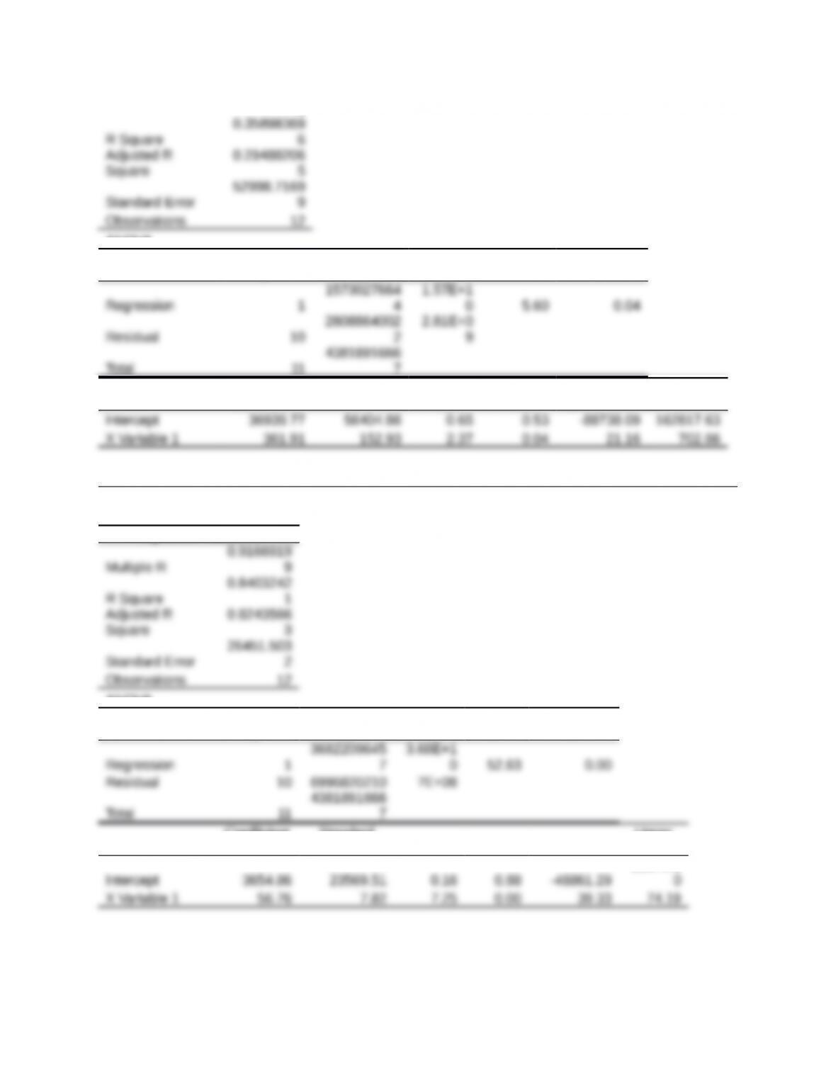
Regression 1: Medical supplies costs = a + (b Number of procedures)
Variable Coefficient Standard
Error
t-Value
Constant $36,939.77 $56,404.86 0.65
Independent variable: No. of procedures $ 361.91 $ 152.93 2.37
r2 = 0.36; Durbin-Watson statistic = 2.48
Regression 2: Medical supplies costs = a + (b Number of patient-hours)
Variable Coefficient Standard Error t-Value
Constant $3,654.86 $23,569.51 0.16
Independent variable: No. of patient-hours $ 56.76 $ 7.82 7.25
r2 = 0.84; Durbin-Watson statistic = 1.91
2. On different graphs plot the data and the regression lines for each of the following cost
functions:
a. Medical supplies costs = a + (b Number of procedures)
b. Medical supplies costs = a + (b Number of patient-hours)
3. Evaluate the regression models for “Number of procedures” and “Number of patient-hours”
as the cost driver according to the format of Exhibit 10-18 (page 406).
4. Based on your analysis, which cost driver should Julie Chen adopt for Apollo Hospital?
Explain your answer.
SOLUTION
(30 min.) Regression; choosing among models.
1. See Solution Exhibit 10-42A below.
SOLUTION EXHIBIT 10-42A
(a) Regression Output for Medical Supplies Costs and Number of Procedures
SUMMARY OUTPUT
Regression Statistics
Multiple R 0.59915248
10-5
1
ANOVA
df SS MS F
Significance
F
Total 11
7
Coefficients
Standard
Error t Stat P-value Lower 95%
Upper
95%
(b) Regression Output for Medical Supplies Costs and Number of Patient-Hours
SUMMARY OUTPUT
Regression Statistics
ANOVA
df SS MS F
Significance
F
Coefficient
s
Standard
Error t Stat P-value Lower 95%
Upper
95%
56171.0
2. See Solution Exhibit 10-42B below.
SOLUTION EXHIBIT 10-42B
10-6
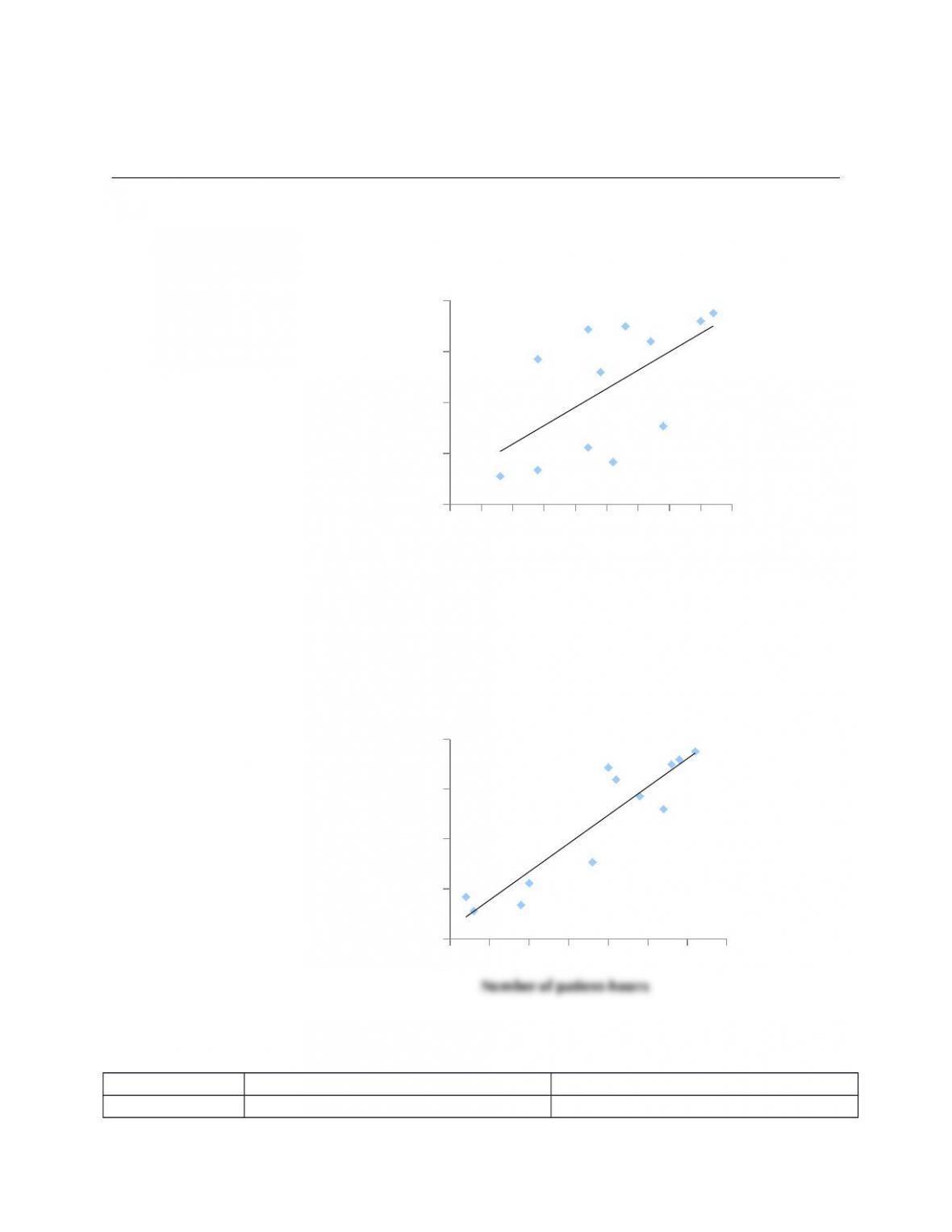
Plots and Regression Lines for (a) Medical Supplies Costs and Number of Procedures and (b)
Medical Supplies Costs and Number of Patient-Hours
(a)
100 150 200 250 300 350 400 450 500 550
50,000
100,000
150,000
200,000
250,000
f(x) = 361.91x + 36939.77
R² = 0.36
Apollo Hospitals
Number of procedures
Medical supplies costs
(b)
1,000 1,500 2,000 2,500 3,000 3,500 4,000 4,500
50,000
100,000
150,000
200,000
250,000
f(x) = 56.76x + 3654.86
R² = 0.84
Apollo Hospitals
Medical supplies costs
3.
Number of Setups Number of Setup Hours
Economic A positive relationship A positive relationship between
10-7
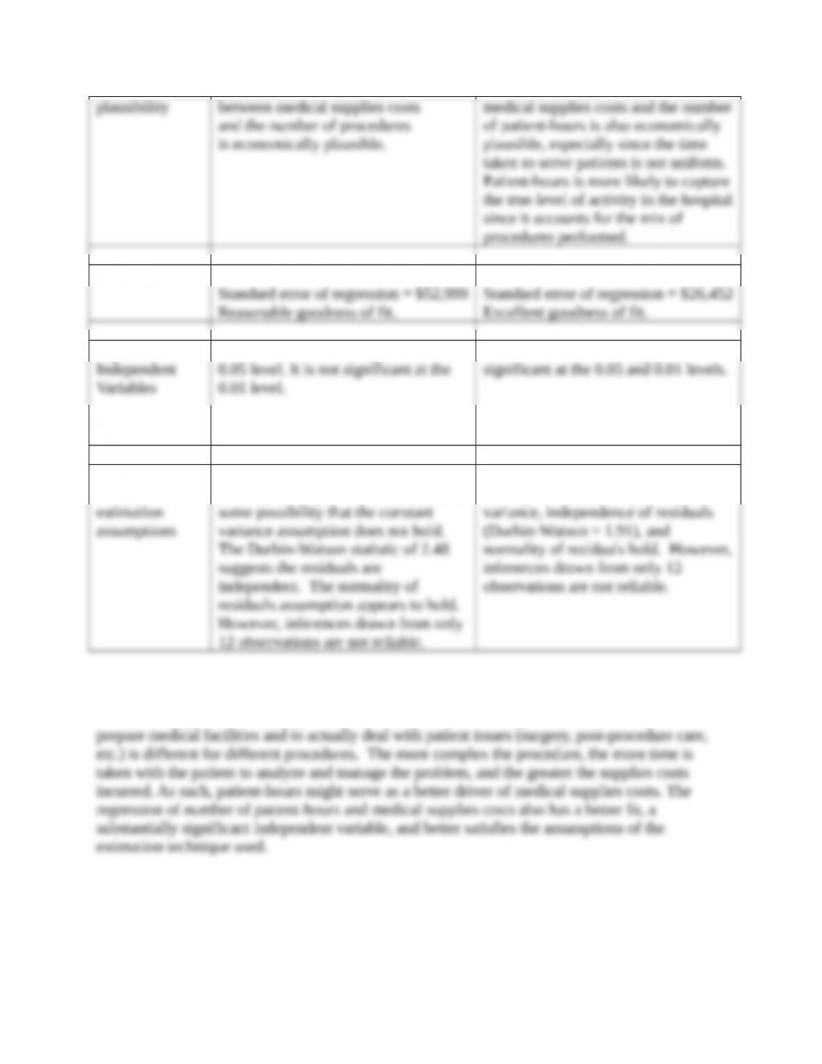
Goodness of fit r2 = 36%
r2 = 84%
Significance of
The t-value of 2.37 is significant at the
The t-value of 7.25 is highly
Specification
analysis of
Based on a plot of the data, the
linearity assumption holds, but there is
Based on a plot of the data, the
assumptions of linearity, constant
4. The regression model using number of patient-hours should be used to estimate medical
supplies costs because the number of patient-hours is a more economically plausible cost driver
of medical supplies costs (compared to the number of procedures performed). The time taken to
10-43 Multiple regression (continuation of 10-42). After further discussion,
Julie and Rhett wonder if they should view both the number of procedures and number of
patient-hours as cost drivers in a multiple regression estimation in order to best understand
Apollo’s medical supplies costs.
10-8

Required:
1. Conduct a multiple regression to estimate the regression equation for medical supplies costs
using both number of procedures and number of patient-hours as independent variables. You
should obtain the following result:
Regression 3: Medical supplies costs = a + (b1 No. of procedures) + (b2 No. of
patient-hours)
Variable Coefficient Standard Error t-Value
Constant –$3,103.76 $30,406.54 –0.10
Independent variable 1: No. of procedures $ 38.24 $ 100.76 0.38
Independent variable 2: No. of patient-hours $ 54.37 $ 10.33 5.26
r2 = 0.84; Durbin-Watson statistic = 1.96
2. Evaluate the multiple regression output using the criteria of economic plausibility goodness
of fit, significance of independent variables, and specification of estimation assumptions.
3. What potential issues could arise in multiple regression analysis that are not present in simple
regression models? Is there evidence of such difficulties in the multiple regression presented
in this problem? Explain.
4. Which of the regression models from Problems 10-42 and 10-43 would you recommend Julie
Chen use? Explain.
10-9