SOLUTION
(15-20min.) Interpreting regression results, matching time periods.
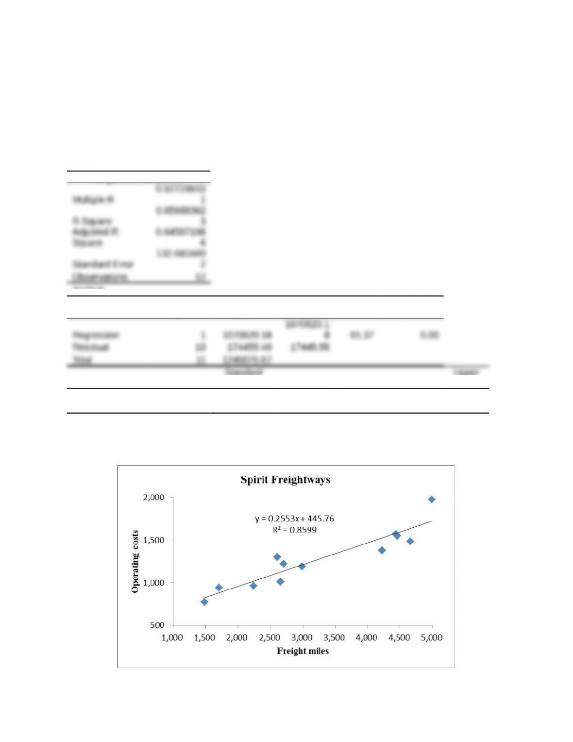
1. Here is the regression data for monthly operating costs as a function of the total freight
miles travelled by Sprit vehicles:
SUMMARY OUTPUT
Regression Statistics
ANOVA
df SS MS F
Significance
F
Coefficients
Standard
Error t Stat P-value Lower 95%
Upper
95%
Intercept 445.76 112.97 3.95 0.00 194.04 697.48
X Variable 1 0.26 0.03 7.83 0.00 0.18 0.33
2. The chart below presents the data and the estimated regression line for the relationship
between monthly operating costs and freight miles traveled by Spirit Freightways.
10-1
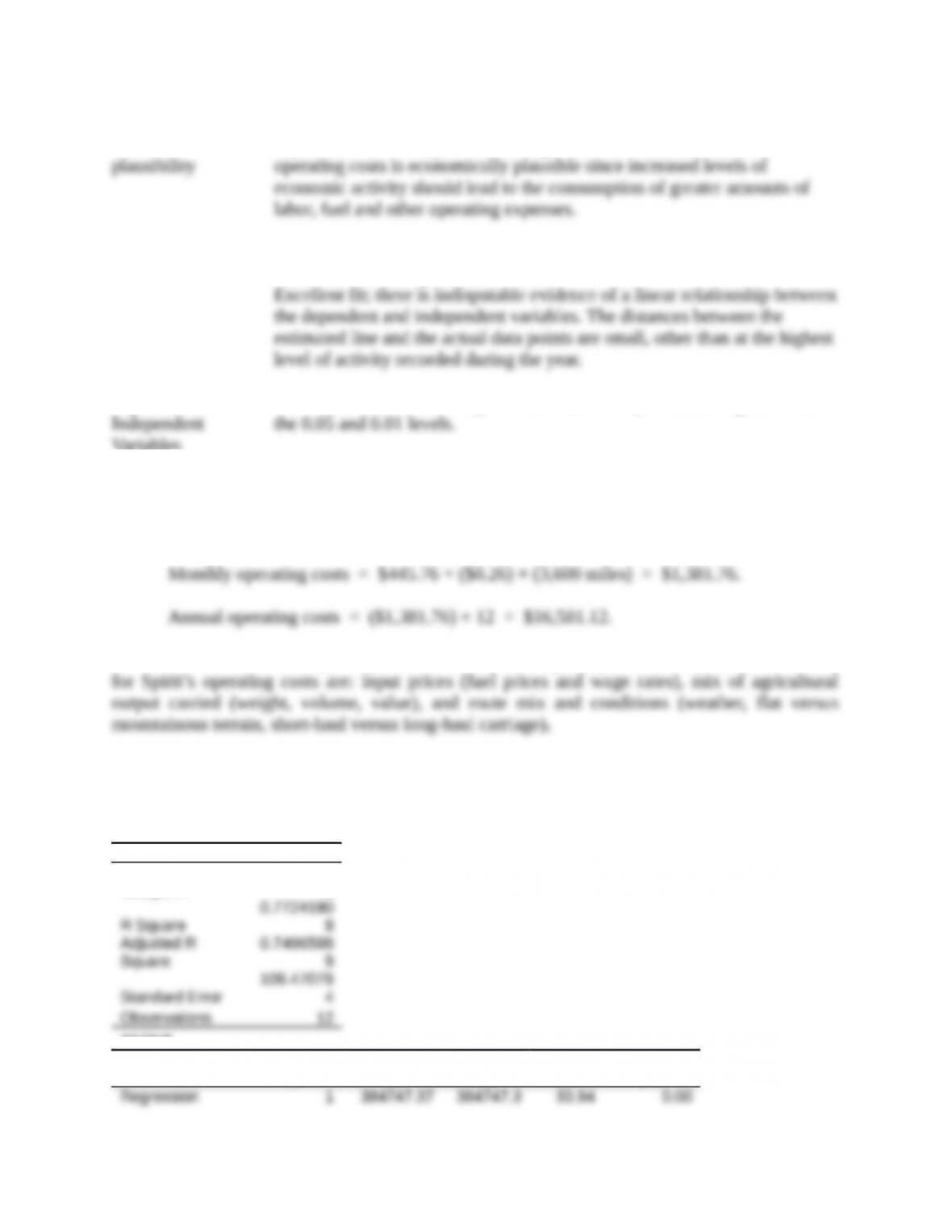
Economic
A positive relationship between freight miles traveled and monthly
Goodness of fit r2 = 86%, Adjusted r2 = 85%
Standard error of regression = 132.08
Significance of
Variables
The t-value of 7.83 for freight miles traveled output units is significant at
3. If Brown expects Spirit to generate an average of 3,600 miles each month next year, the best
estimate of operating costs is given by:
4. Three variables, other than freight miles, that Brown might expect to be important cost drivers
5. Here is the regression data for monthly maintenance costs as a function of the total freight
miles travelled by Sprit vehicles:
SUMMARY OUTPUT
Regression Statistics
Multiple R
0.8788731
9
ANOVA
df SS MS F
Significanc
e F
10-2
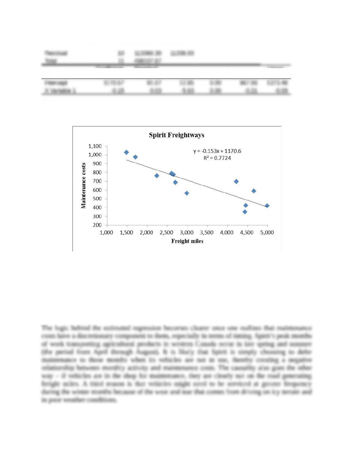
7
Coefficient
s
Standard
Error t Stat P-value Lower 95%
Upper
95%
The data and regression estimate are provided in the chart below:
6. At first glance, the regression result in requirement 5 is surprising and
economically-implausible. In the regression, the coefficient on freight miles traveled has a
negative sign. This implies that the greater the number of freight miles (i.e., the more activity
Spirit carries out), the smaller are the maintenance costs; specifically, it suggests that each extra
freight mile reduces maintenance costs by $0.14 (recall that all data are in thousands). Clearly,
this estimated relationship is not economically credible. However, one would think that freight
miles should have some impact on fleet maintenance costs.
10-3
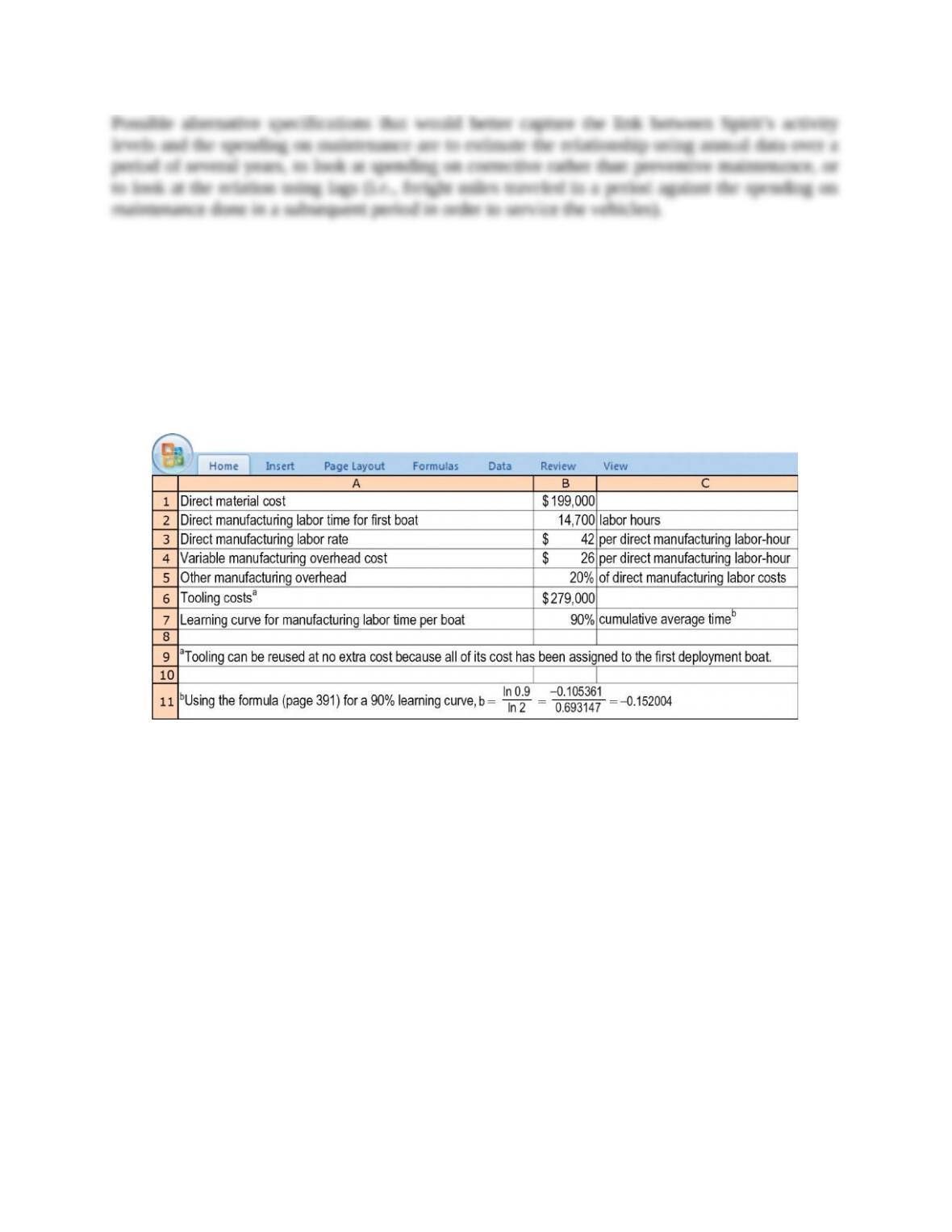
10-40 Cost estimation, cumulative average-time learning curve. The
Pacific Boat Company, which is under contract to the U.S. Navy, assembles troop deployment
boats. As part of its research program, it completes the assembly of the first of a new model
(PT109) of deployment boats. The Navy is impressed with the PT109. It requests that Pacific
Boat submit a proposal on the cost of producing another six PT109s.
Pacific Boat reports the following cost information for the first PT109 assembled and uses a
90% cumulative average-time learning model as a basis for forecasting direct manufacturing
labor-hours for the next six PT109s. (A 90% learning curve means b = –0.152004.)
Required:
1. Calculate predicted total costs of producing the six PT109s for the Navy. (Pacific Boat will
keep the first deployment boat assembled, costed at $1,477,600, as a demonstration model
for potential customers.)
2. What is the dollar amount of the difference between (a) the predicted total costs for
producing the six PT109s in requirement 1 and (b) the predicted total costs for producing the
six PT109s, assuming that there is no learning curve for direct manufacturing labor? That is,
for (b) assume a linear function for units produced and direct manufacturing labor-hours.
10-4