SOLUTION
(30min.) High-low method and regression analysis.
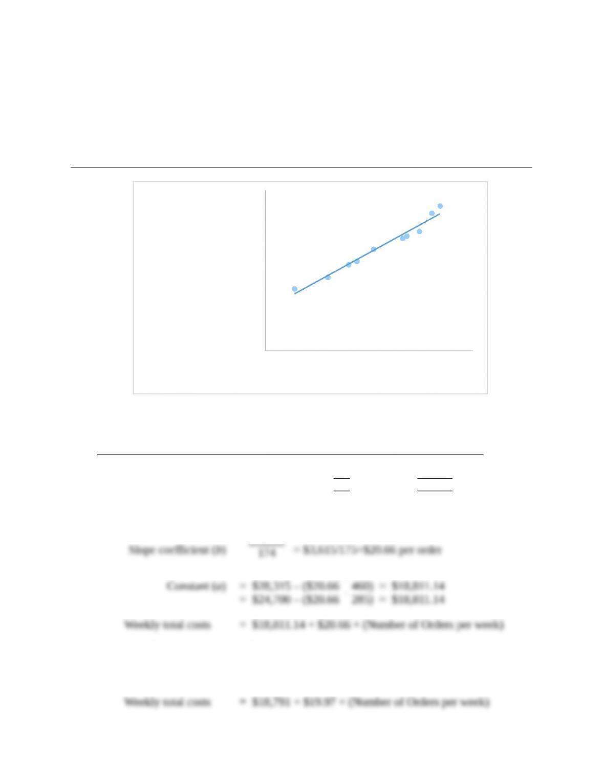
1. See Solution Exhibit 10-36.
SOLUTION EXHIBIT 10-36
250 300 350 400 450 500
$22,000
$23,000
$24,000
$25,000
$26,000
$27,000
$28,000
$29,000
Number of Weekly Orders
Weekly Total Costs
2.
Number of
Orders per week
Weekly
Total Costs
Highest observation of cost driver (Week 8) 460 $28,315
Lowest observation of cost driver (Week 3) 285 24,700
Difference 175 $ 3,615
Weekly total costs = a + b (number of orders per week)
$7,010
See high-low line in Solution Exhibit 10-36.
3. Solution Exhibit 10-36 presents the regression line:
10-1
4. Profit =
Total weekly revenues + Total seasonal membership fees – Total weekly costs
5. Let the average number of weekly orders be denoted by AWO. We want to find the value
of AWO for which Market Thyme will achieve zero profit.
Using the format in requirement 4, we want:
10-37 High-low method; regression analysis. (CIMA, adapted) Catherine
McCarthy, sales manager of Baxter Arenas, is checking to see if there is any relationship
between promotional costs and ticket revenues at the sports stadium. She obtains the following
data for the past 9 months:
10-2

Month Ticket Revenues Promotional Costs
April $200,000 $52,000
May 270,000 65,000
June 320,000 80,000
July 480,000 90,000
August 430,000 100,000
September 450,000 110,000
October 540,000 120,000
November 670,000 180,000
December 751,000 197,000
She estimates the following regression equation:
Ticket revenues = $65,583 + ($3.54 Promotional costs)
Required:
1. Plot the relationship between promotional costs and ticket revenues. Also draw the regression
line and evaluate it using the criteria of economic plausibility, goodness of fit, and slope of
the regression line.
2. Use the high-low method to compute the function relating promotional costs and revenues.
3. Using (a) the regression equation and (b) the high-low equation, what is the increase in
revenues for each $10,000 spent on promotional costs within the relevant range? Which
method should Catherine use to predict the effect of promotional costs on ticket revenues?
Explain briefly.
SOLUTION
(3040 min.) High-low method, regression analysis.
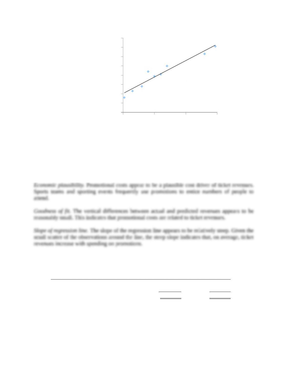
1. Solution Exhibit 10-37 presents the plots of promotional costs on revenues.
SOLUTION EXHIBIT 10-37
Plot and Regression Line of Promotional Costs on Ticket Revenues
10-3
50,000 100,000 150,000 200,000
40,000
140,000
240,000
340,000
440,000
540,000
640,000
740,000
840,000
f(x) = 3.54x + 65582.7
R² = 0.93
Promotional Costs
Ticket Revenues
Solution Exhibit 10-37 also shows the regression line of advertising costs on revenues.
We evaluate the estimated regression equation using the criteria of economic plausibility,
goodness of fit, and slope of the regression line.
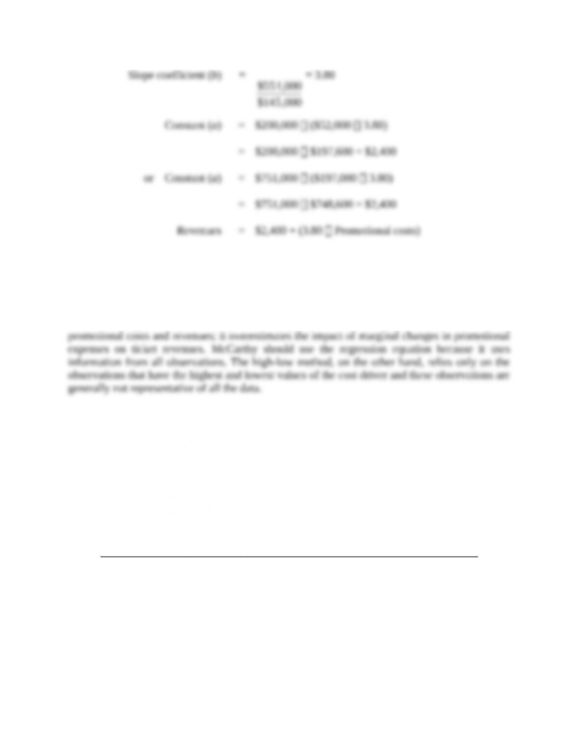
2. The high-low method would estimate the cost function as follows:
Promotional Ticket
Costs Revenues
Highest observation of revenue driver $ 52,000 $200,000
Lowest observation of revenue driver 197,000 751,000
Difference $145,000 $551,000
Revenues = a + (b promotional costs)
10-4
3. The increase in revenues for each $1,000 spent on advertising within the relevant range is
a. Using the regression equation, 3.542 $10,000 = $35,420
b. Using the high-low equation, 3.80 $10,000 = $38,000
The high-low equation does moderately well in estimating the relationship between
10-38 Regression, activity-based costing, choosing cost drivers. Sleep
Late, a large hotel chain, has been using activity-based costing to determine the cost of a night’s
stay at their hotels. One of the activities, “Inspection,” occurs after a customer has checked out of
a hotel room. Sleep Late inspects every 10th room and has been using “number of rooms
inspected” as the cost driver for inspection costs. A significant component of inspection costs is
the cost of the supplies used in each inspection.
Mary Adams, the chief inspector, is wondering whether inspection labor-hours might be a
better cost driver for inspection costs. Mary gathers information for weekly inspection costs,
rooms inspected, and inspection labor-hours as follows:
Week Rooms Inspected Inspection Labor-Hours Inspection Costs
1 254 66 $1,740
2 322 110 2,500
3 335 82 2,250
4 431 123 2,800
5 198 48 1,400
6 239 62 1,690
10-5
Week Rooms Inspected Inspection Labor-Hours Inspection Costs
7 252 108 1,720
8 325 127 2,200
Mary runs regressions on each of the possible cost drivers and estimates these cost functions:
Inspection Costs = $193.19 + ($6.26 Number of rooms inspected)
Inspection Costs = $944.66 + ($12.04 Inspection labor-hours)
Required:
1. Explain why rooms inspected and inspection labor-hours are plausible cost drivers of
inspection costs.
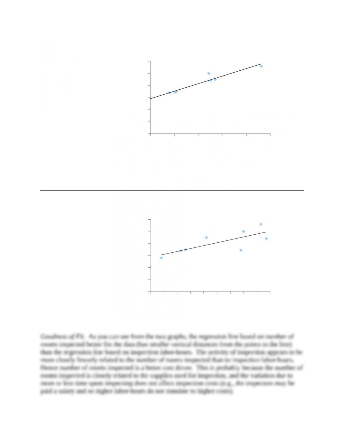
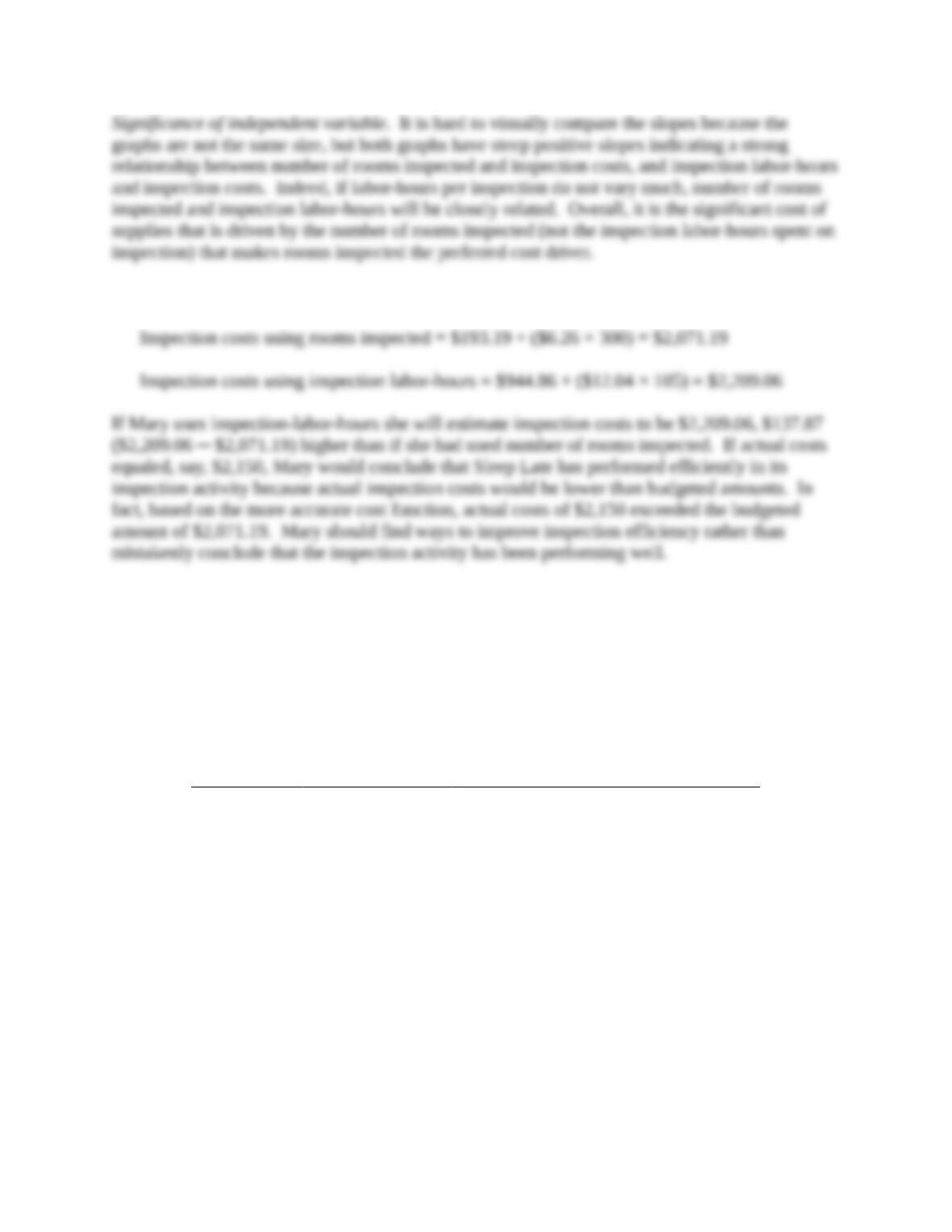
2. Plot the data and regression line for rooms inspected and inspection costs. Plot the data and
regression line for inspection labor-hours and inspection costs. Which cost driver of
inspection costs would you choose? Explain.
3. Mary expects inspectors to inspect 300 rooms and work for 105 hours next week. Using the
cost driver you chose in requirement 2, what amount of inspection costs should Mary
budget? Explain any implications of Mary choosing the cost driver you did not choose in
requirement 2 to budget inspection costs.
SOLUTION
(30 min.) Regression, activity-based costing, choosing cost drivers.
1. Both number of rooms inspected and inspection labor-hours are plausible cost drivers for
inspection costs. The number of rooms inspected is likely related to the materials and supplies
2. Solution Exhibit 10-38 presents (a) the plots and regression line for number of rooms
SOLUTION EXHIBIT 10-38A
Plot and Regression Line for Rooms Inspected versus Inspection Costs for Sleep Late
10-6
200 250 300 350 400 450
$0
$500
$1,000
$1,500
$2,000
$2,500
$3,000
f(x) = 6.26x + 193.19
R² = 0.94
Sleep Late
Rooms inspected
Inspecon costs
SOLUTION EXHIBIT 10-38B
Plot and Regression Line for Inspection Labor-Hours and Inspection Costs for Sleep Late
40 50 60 70 80 90 100 110 120 130
$0
$500
$1,000
$1,500
$2,000
$2,500
$3,000
f(x) = 12.04x + 944.66
R² = 0.58
Sleep Late
Inspection labor-hours
Inspection costs
10-7
3. At 105 inspection labor hours and 300 rooms inspected:
10-39 Interpreting regression results. Spirit Freightways is a leader in transporting
agricultural products in the western provinces of Canada. Reese Brown, a financial analyst at Spirit
Freightways, is studying the behavior of transportation costs for budgeting purposes. Transportation
costs at Spirit are of two types: (a) operating costs (such as labor and fuel) and (b) maintenance
costs (primarily overhaul of vehicles).
Brown gathers monthly data on each type of cost, as well as the total freight miles traveled
by Spirit vehicles in each month. The data collected are shown below (all in thousands):
Month Operating Costs Maintenance Costs Freight Miles
January $ 942 $ 974 1,710
February 1,008 776 2,655
March 1,218 686 2,705
April 1,380 694 4,220
May 1,484 588 4,660
June 1,548 422 4,455
July 1,568 352 4,435
August 1,972 420 4,990
September 1,190 564 2,990
October 1,302 788 2,610
November 962 762 2,240
10-8
December 772 1,028 1,490
Required:
1. Conduct a regression using the monthly data of operating costs on freight miles. You should
obtain the following result:
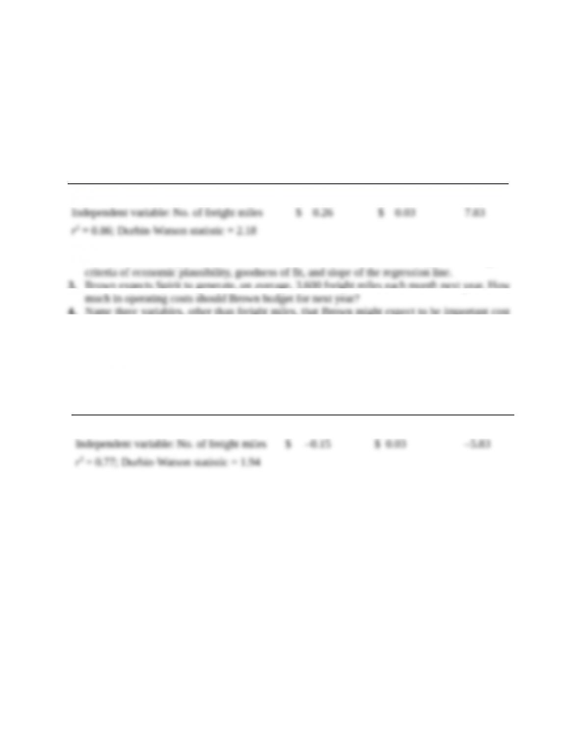
Regression: Operating costs = a + (b Number of freight miles)
Variable Coefficient Standard Error t-Value
Constant $445.76 $112.97 3.95
2. Plot the data and regression line for the above estimation. Evaluate the regression using the
3. Brown expects Spirit to generate, on average, 3,600 freight miles each month next year. How
4. Name three variables, other than freight miles, that Brown might expect to be important cost
drivers for Spirit’s operating costs.
5. Brown next conducts a regression using the monthly data of maintenance costs on freight
miles. Verify that she obtained the following result:
Regression: Maintenance costs = a + (b Number of freight miles)
Variable Coefficient Standard Error t-Value
Constant $1,170.57 $91.07 12.85
6. Provide a reasoned explanation for the observed sign on the cost driver variable in the
maintenance cost regression. What alternative data or alternative regression specifications
would you like to use to better capture the above relationship?
10-9