.SOLUTION
(20 min.) Various cost-behavior patterns.
1. K
2. B
3. G
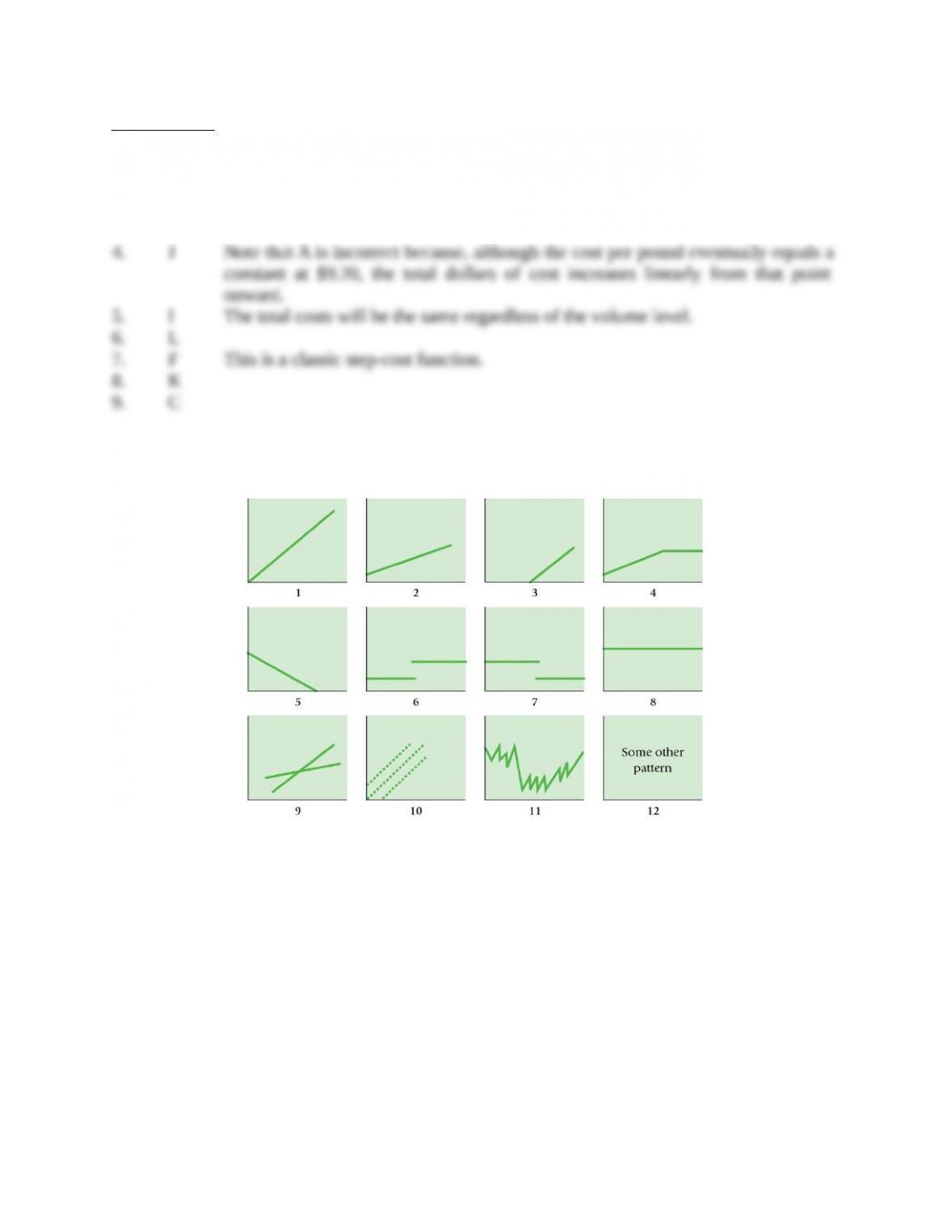
10-24 Matching graphs with descriptions of cost and revenue
behavior. (D. Green, adapted) Given here are a number of graphs.
Required:
The horizontal axis of each graph represents the units produced over the year, and the vertical
axis represents total cost or revenues.
Indicate by number which graph best fits the situation or item described (a–h). Some graphs
may be used more than once; some may not apply to any of the situations.
a. Direct material costs
b. Supervisors’ salaries for one shift and two shifts
c. A cost–volume–profit graph
d. Mixed costs—for example, car rental fixed charge plus a rate per mile driven
e. Depreciation of plant, computed on a straight-line basis
f. Data supporting the use of a variable-cost rate, such as manufacturing labor cost of $14 per unit
produced
10-1
g. Incentive bonus plan that pays managers $0.10 for every unit produced above some level of
production
h. Interest expense on $2 million borrowed at a fixed rate of interest
SOLUTION
(30 min.) Matching graphs with descriptions of cost and revenue behavior.
a. (1)
10-25 Account analysis, high-low. Stein Corporation wants to find an equation to
estimate some of their monthly operating costs for the operating budget for 2018. The following
cost and other data were gathered for 2017:
Month
Maintenance
Costs
Machine
Hours
Health
Insurance
Number of
Employees
Shipping
Costs
Units
Shipped
January $4,500 165 $8,600 68 $25,776 7,160
February $4,452 120 $8,600 75 $29,664 8,240
March $4,600 230 $8,600 92 $28,674 7,965
April $4,850 318 $8,600 105 $23,058 6,405
May $5,166 460 $8,600 89 $21,294 5,915
June $4,760 280 $8,600 87 $33,282 9,245
July $4,910 340 $8,600 93 $31,428 8,730
August $4,960 360 $8,600 88 $30,294 8,415
September $5,070 420 $8,600 95 $25,110 6,975
October $5,250 495 $8,600 102 $25,866 7,185
November $5,271 510 $8,600 97 $20,124 5,590
December $4,760 275 $8,600 94 $34,596 9,610
Required:
1. Which of the preceding costs is variable? Fixed? Mixed? Explain.
2. Using the high-low method, determine the cost function for each cost.
10-2
3. Combine the preceding information to get a monthly operating cost function for the Stein
Corporation.
4. Next month, Stein expects to use 400 machine hours, have 80 employees, and ship 9,000
units. Estimate the total operating cost for the month.
SOLUTION
(20 min.) Account analysis, high-low
1. The maintenance cost is a mixed cost because the cost neither remains constant in total nor
2. The month with the highest number of machine hours is November, with 510 machine hours
and $5,271 of cost. The month with the lowest is February, with 120 machine hours and $4,452
in cost. The difference in cost ($5,271 – $4,452), divided by the difference in machine hours (510
– 120) equals $2.10 per machine hour of variable maintenance cost. Inserted into the cost
formula for November:
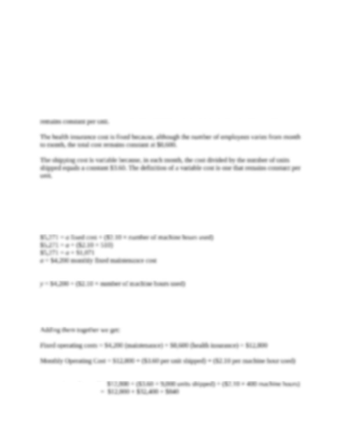
Therefore, Stein’s cost formula for monthly maintenance cost is:
3. The shipping rate is $3.60 per unit shipped
The maintenance cost is $4,200 + ($2.10 per machine hour used)
The health insurance cost is $8,600.
4. Estimated operating cost for November:
10-3

10-26 Account analysis method. Gower, Inc., a manufacturer of plastic products,
reports the following manufacturing costs and account analysis classification for the year ended
December 31, 2017.
Account Classification Amount
Direct materials All variable $300,000
Direct manufacturing labor All variable 225,000
Power All variable 37,500
Supervision labor 20% variable 56,250
Materials-handling labor 50% variable 60,000
Maintenance labor 40% variable 75,000
Depreciation 0% variable 95,000
Rent, property taxes, and administration 0% variable 100,000
Gower, Inc., produced 75,000 units of product in 2017. Gower’s management is estimating costs
for 2018 on the basis of 2017 numbers. The following additional information is available for
2018.
a. Direct materials prices in 2018 are expected to increase by 5% compared with 2017.
b. Under the terms of the labor contract, direct manufacturing labor wage rates are expected to
increase by 10% in 2018 compared with 2017.
c. Power rates and wage rates for supervision, materials handling, and maintenance are not
expected to change from 2017 to 2018.
d. Depreciation costs are expected to increase by 5%, and rent, property taxes, and
administration costs are expected to increase by 7%.
e. Gower expects to manufacture and sell 80,000 units in 2018.
Required:
1. Prepare a schedule of variable, fixed, and total manufacturing costs for each account category
in 2018. Estimate total manufacturing costs for 2018.
2. Calculate Gower’s total manufacturing cost per unit in 2017, and estimate total
manufacturing cost per unit in 2018.
3. How can you obtain better estimates of fixed and variable costs? Why would these better
estimates be useful to Gower?
SOLUTION
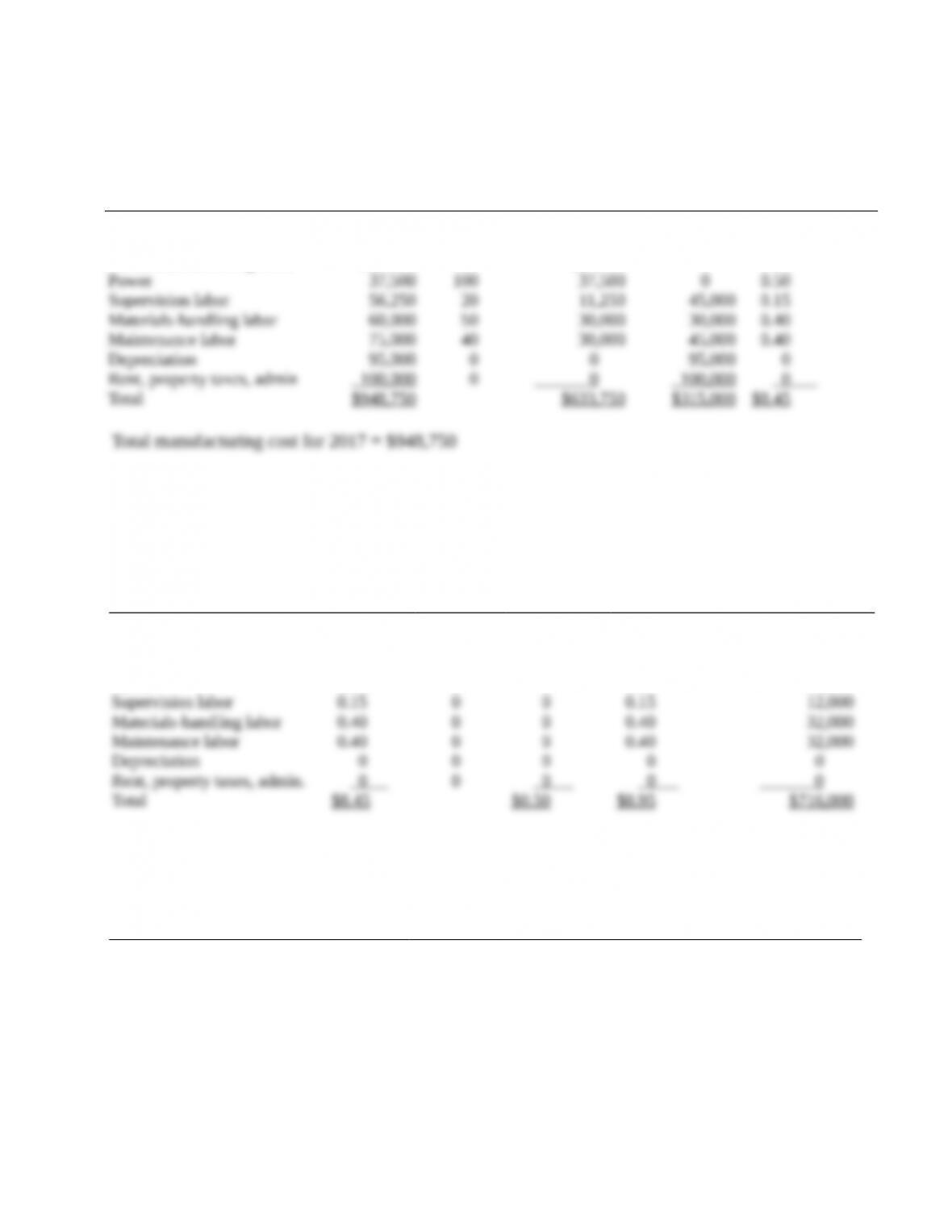
(30 min.) Account analysis method.
1. Manufacturing cost classification for 2017:
10-4
Account
Total
Costs
(1)
% of
Total Costs
That is
Variable
(2)
Variable
Costs
(3) = (1) (2)
Fixed
Costs
(4) = (1) – (3)
Variable
Cost per Unit
(5) = (3) ÷ 75,000
Direct materials
Direct manufacturing labor
$300,000
225,000
100%
100
$300,000
225,000
$ 0
0
$4.00
3.00
Variable costs in 2018:
Account
Unit
Variable
Cost per
Unit for
2017
(6)
Percentage
Increase
(7)
Increase in
Variable
Cost
per Unit
(8) = (6) (7)
Variable Cost
per Unit
for 2018
(9) = (6) + (8)
Total Variable
Costs for 2018
(10) = (9) 80,000
Direct materials
Direct manufacturing labor
Power
$4.00
3.00
0.50
5%
10
0
$0.20
0.30
0
$4.20
3.30
0.50
$336,000
264,000
40,000
Fixed and total costs in 2018:
Account
Fixed
Costs
for 2018
(11)
Percentage
Increase
(12)
Dollar
Increase in
Fixed Costs
(13) =
(11) (12)
Fixed Costs
for 2018
(14) =
(11) + (13)
Variable
Costs for
2018
(15)
Total
Costs
(16) =
(14) + (15)
10-5
Direct materials
Direct manufacturing labor
Power
Supervision labor
$ 0
0
0
45,000
0%
0
0
0
$ 0
0
0
0
$ 0
0
0
45,000
$336,000
264,000
40,000
12,000
$ 336,000
264,000
40,000
57,000
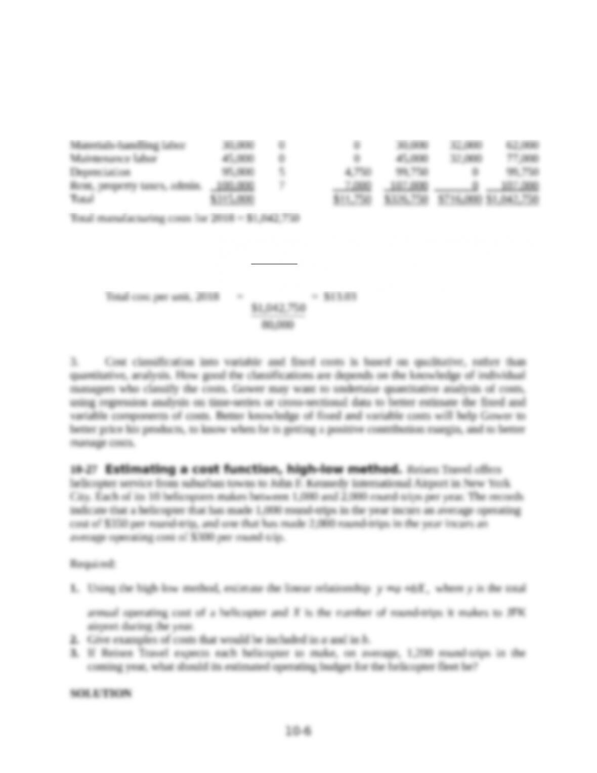
2. Total cost per unit, 2017 =
75,000
$948,750
= $12.65
80,000
$1,042,750
3. Cost classification into variable and fixed costs is based on qualitative, rather than
quantitative, analysis. How good the classifications are depends on the knowledge of individual
10-27 Estimating a cost function, high-low method. Reisen Travel offers
helicopter service from suburban towns to John F. Kennedy International Airport in New York
City. Each of its 10 helicopters makes between 1,000 and 2,000 round-trips per year. The records
indicate that a helicopter that has made 1,000 round-trips in the year incurs an average operating
cost of $350 per round-trip, and one that has made 2,000 round-trips in the year incurs an
average operating cost of $300 per round-trip.
Required:
1. Using the high-low method, estimate the linear relationship
,y a bX= +
where y is the total
annual operating cost of a helicopter and X is the number of round-trips it makes to JFK
airport during the year.
2. Give examples of costs that would be included in a and in b.
3. If Reisen Travel expects each helicopter to make, on average, 1,200 round-trips in the
coming year, what should its estimated operating budget for the helicopter fleet be?
SOLUTION
10-6
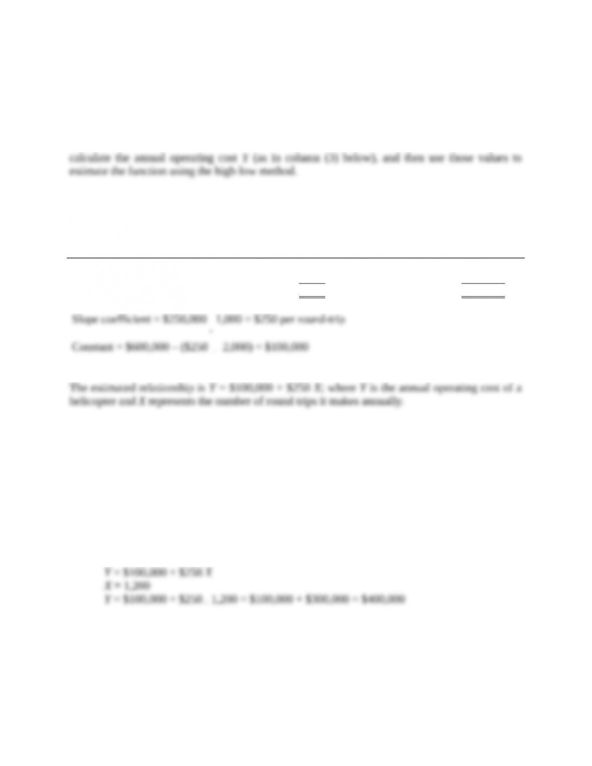
(15–20 min.) Estimating a cost function, high-low method.
1. The key point to note is that the problem provides high-low values of X (annual round
trips made by a helicopter) and Y
¸
X (the operating cost per round trip). We first need to
Cost Driver:
Annual Round-
Trips (X)
Operating
Cost per
Round-Trip
Annual
Operating
Cost (Y)
(1) (2)
(3) = (1)
´
(2)
Highest observation of cost driver 2,000 $300 $600,000
Lowest observation of cost driver 1,000 $350 $350,000
Difference 1,000 $250,000
´
2. The constant a (estimated as $100,000) represents the fixed costs of operating a
helicopter, irrespective of the number of round trips it makes. This would include items such as
insurance, registration, depreciation on the aircraft, and any fixed component of pilot and crew
salaries. The coefficient b (estimated as $250 per round-trip) represents the variable cost of each
round trip—costs that are incurred only when a helicopter actually flies a round trip. The
coefficient b may include costs such as landing fees, fuel, refreshments, baggage handling, and
any regulatory fees paid on a per-flight basis.
3. If each helicopter is, on average, expected to make 1,200 round trips a year, we can use
the estimated relationship to calculate the expected annual operating cost per helicopter:
´
With 10 helicopters in its fleet, Reisen’s estimated operating budget is 10
´
$400,000 = $4,000,000.
10-7
10-28 Estimating a cost function, high-low method. Lacy Dallas is examining
customer-service costs in the southern region of Camilla Products. Camilla Products has more
than 200 separate electrical products that are sold with a 6-month guarantee of full repair or
replacement with a new product. When a product is returned by a customer, a service report is
prepared. This service report includes details of the problem and the time and cost of resolving
the problem. Weekly data for the most recent 8-week period are as follows:
Week Customer-Service Department Costs Number of Service Reports
1 $13,300 185
2 20,500 285
3 12,000 120
4 18,500 360
5 14,900 275
6 21,600 440
7 16,500 350
8 21,300 315
Required:
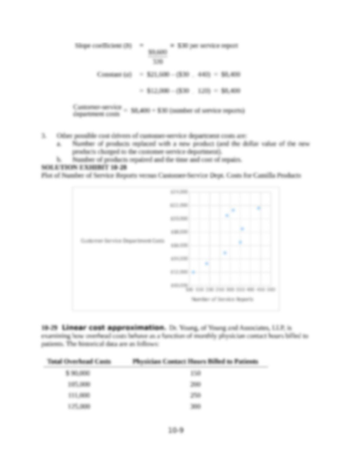
1. Plot the relationship between customer-service costs and number of service reports. Is the
relationship economically plausible?
2. Use the high-low method to compute the cost function relating customer-service costs to the
number of service reports.
3. What variables, in addition to number of service reports, might be cost drivers of weekly
customer-service costs of Camilla Products?
SOLUTION
(20 min.) Estimating a cost function, high-low method.
1. See Solution Exhibit 10-28. There is a positive relationship between the number of
service reports (a cost driver) and the customer-service department costs. This relationship is
economically plausible.
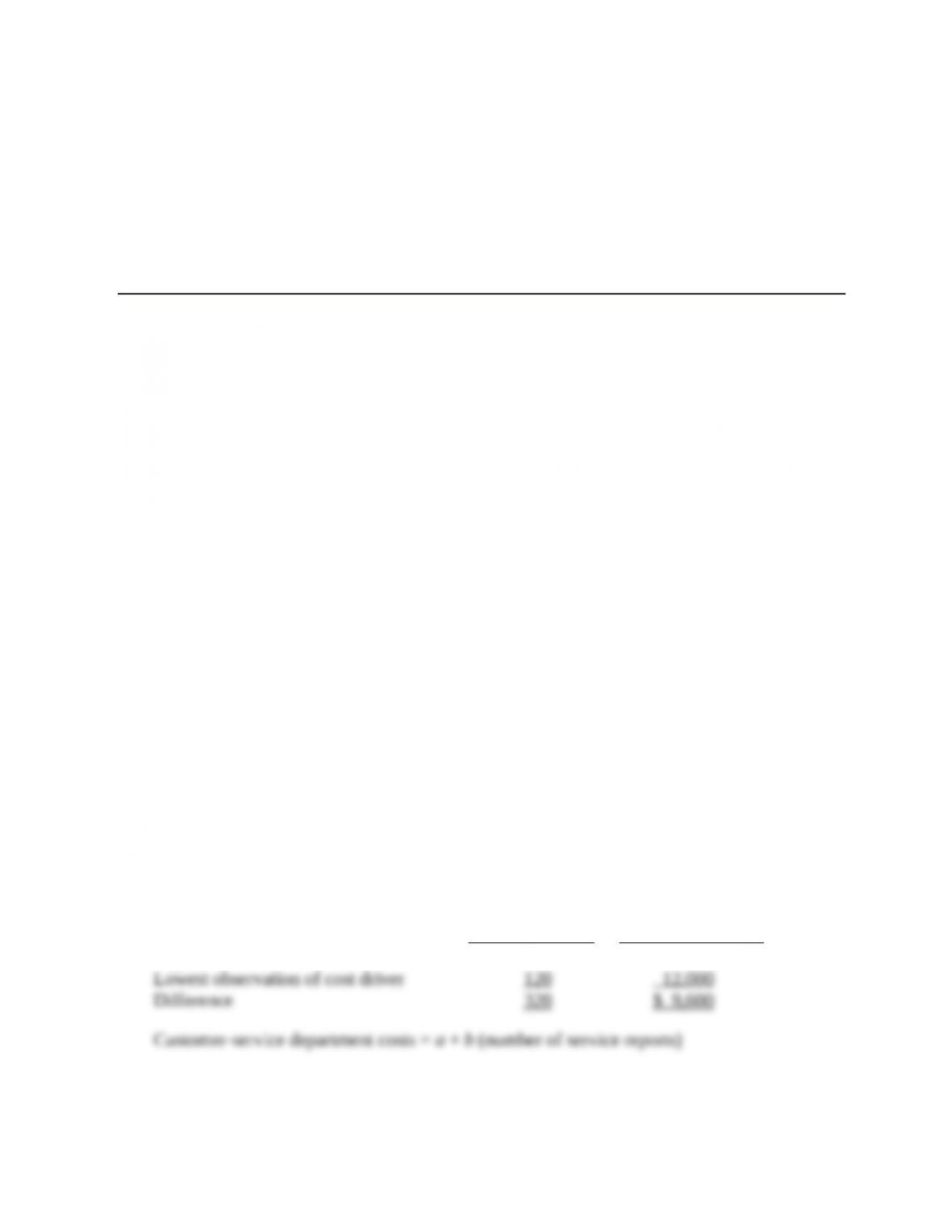
2. Number of Customer-Service
Service Reports Department Costs
Highest observation of cost driver 440 $21,600
10-8
Total Overhead Costs Physician Contact Hours Billed to Patients
137,000 350
150,000 400
Required:
1. Compute the linear cost function, relating total overhead costs to physician contact hours,
using the representative observations of 200 and 300 hours. Plot the linear cost function.
Does the constant component of the cost function represent the fixed overhead costs of
Young and Associates? Why?
2. What would be the predicted total overhead costs for (a) 150 hours and (b) 400 hours using
the cost function estimated in requirement 1? Plot the predicted costs and actual costs for 150
and 400 hours.
3. Dr. Young had a chance to do some school physicals that would have boosted physician
contact hours billed to patients from 200 to 250 hours. Suppose Dr. Young, guided by the
linear cost function, rejected this job because it would have brought a total increase in
contribution margin of $9,000, before deducting the predicted increase in total overhead cost,
$10,000. What is the total contribution margin actually forgone?
SOLUTION
(30–40 min.) Linear cost approximation.
1. Slope coefficient (b) =
Difference in overhead costs
Difference in contact hours billed
No, the constant component of the cost function does not represent the fixed overhead cost of
Young and Associates. The relevant range of physician contact hours billed is from 150 to 400.
The constant component provides the best available starting point for a straight line that
approximates how a cost behaves within the relevant range.
2. A comparison at various levels of contact hours billed follows. The linear cost function is
based on the formula of $65,000 per month plus $200 per physician contact hours billed.
10-10
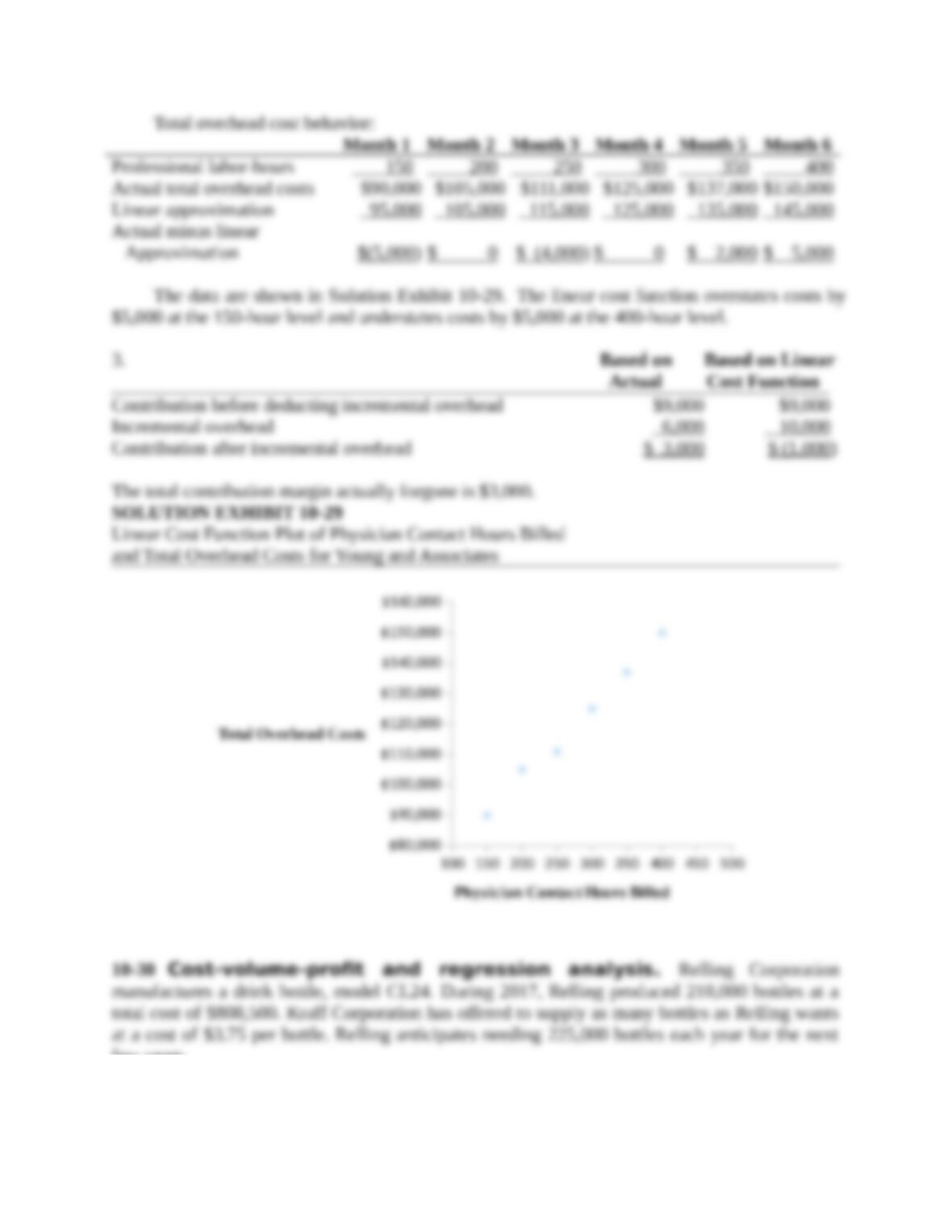
Total overhead cost behavior:
Month 1 Month 2 Month 3 Month 4 Month 5 Month 6
3. Based on Based on Linear
Actual Cost Function
The total contribution margin actually forgone is $3,000.
SOLUTION EXHIBIT 10-29
Linear Cost Function Plot of Physician Contact Hours Billed
and Total Overhead Costs for Young and Associates
100 150 200 250 300 350 400 450 500
$80,000
$90,000
$100,000
$110,000
$120,000
$130,000
$140,000
$150,000
$160,000
Physician Contact Hours Billed
Total Overhead Costs
10-30 Cost-volume-pro!t and regression analysis. Relling Corporation
manufactures a drink bottle, model CL24. During 2017, Relling produced 210,000 bottles at a
total cost of $808,500. Kraff Corporation has offered to supply as many bottles as Relling wants
few years.
Required:
10-11
1. a. What is the average cost of manufacturing a drink bottle in 2017? How does it compare to
Kraff’s offer?
b. Can Relling use the answer in requirement 1a to determine the cost of manufacturing
225,000 drink bottles? Explain.
2. Relling’s cost analyst uses annual data from past years to estimate the following regression