CHAPTER 10
DETERMINING HOW COSTS BEHAVE
10-1 What two assumptions are frequently made when estimating a cost function?
The two assumptions are
1. Variations in the level of a single activity (the cost driver) explain the variations in the
2. Cost behavior is approximated by a linear cost function within the relevant range. A
10-2 Describe three alternative linear cost functions.
Three alternative linear cost functions are
1. Variable cost function––a cost function in which total costs change in proportion to the
changes in the level of activity in the relevant range.
10-3 What is the difference between a linear and a nonlinear cost function? Give an example
of each type of cost function.
A linear cost function is a cost function where, within the relevant range, the graph of total costs
versus the level of a single activity related to that cost is a straight line. An example of a linear
10-4 “High correlation between two variables means that one is the cause and the other is the
effect.” Do you agree? Explain.
No. High correlation merely indicates that the two variables move together in the data examined.
10-5 Name four approaches to estimating a cost function.
Four approaches to estimating a cost function are
10-1
1. Industrial engineering method.
2. Conference method.
3. Account analysis method.
4. Quantitative analysis of current or past cost relationships.
10-6 Describe the conference method for estimating a cost function. What are two advantages
of this method?
The conference method estimates cost functions on the basis of analysis and opinions about costs
and their drivers gathered from various departments of a company (purchasing, process
engineering, manufacturing, employee relations, etc.). Advantages of the conference method
include
1. The speed with which cost estimates can be developed.
2. The pooling of knowledge from experts across functional areas.
3. The improved credibility of the cost function to all personnel.
10-7 Describe the account analysis method for estimating a cost function.
10-8 List the six steps in estimating a cost function on the basis of an analysis of a past cost
relationship. Which step is typically the most difficult for the cost analyst?
The six steps are
1. Choose the dependent variable (the variable to be predicted, which is some type of cost).
10-9 When using the high-low method, should you base the high and low observations on the
dependent variable or on the cost driver?
10-10 Describe three criteria for evaluating cost functions and choosing cost drivers.
Three criteria important when choosing among alternative cost functions are
1. Economic plausibility.
10-2
2. Goodness of fit.
3. Slope of the regression line.
10-11 Define learning curve. Outline two models that can be used when incorporating learning
into the estimation of cost functions.
A learning curve is a function that measures how labor-hours per unit decline as units of
production increase because workers are learning and becoming better at their jobs. Two models
used to capture different forms of learning are
10-12 Discuss four frequently encountered problems when collecting cost data on variables
included in a cost function.
Frequently encountered problems when collecting cost data on variables included in a cost
function are
1. The time period used to measure the dependent variable is not properly matched with the
time period used to measure the cost driver(s).
10-13 What are the four key assumptions examined in specification analysis in the case of
simple regression?
Four key assumptions examined in specification analysis are
1. Linearity of relationship between the dependent variable and the independent variable
within the relevant range.
10-14 “All the independent variables in a cost function estimated with regression analysis are
cost drivers.” Do you agree? Explain.
10-3
to maximize goodness of fit, irrespective of the economic plausibility of the independent
variables included. Some of the independent variables included may not be cost drivers.
10-15 “Multicollinearity exists when the dependent variable and the independent variable are
highly correlated.” Do you agree? Explain.
No. Multicollinearity exists when two or more independent variables are highly correlated with
each other.
10-16 HL Co. uses the high-low method to derive a total cost formula. Using a range of units
produced from 1,500 to 7,500, and a range of total costs from $21,000 to $45,000, producing
2,000 units will cost HL:
a. $8,000 b. $12,000
c. $23,000 d. $29,000
SOLUTION
Choice “c” is correct. The high-low method is used to estimate both fixed and variable costs, and
can then be applied to determine a total cost formula that is used to estimate total costs for any
level of production.
10-17 A firm uses simple linear regression to forecast the costs for its main product line. If fixed
costs are equal to $235,000 and variable costs are $10 per unit, how many units does it need to
sell at $15 per unit to make a $300,000 profit?
10-4
a. 21,400 b. 47,000
c. 60,000 d. 107,000
SOLUTION
Choice “d” is correct. The regression equation set up will be: y (total costs) = $235,000 + $10x,
with x representing volume. In order to make a $300,000 profit, sales ($15x) − costs must equal
$300,000. So the full set up will be: $15x − ($235,000 + $10x) = $300,000. Solving for x, $5x =
$535,000, or 107,000 units. At 107,000 units, sales will total $1,605,000 and costs will total
$1,305,000 for a profit of $300,000.
10-18 In regression analysis, the coefficient of determination:
a. Is used to determine the proportion of the total variation in the dependent variable (y)
explained by the independent variable (X).
b. Ranges between negative one and positive one.
c. Is used to determine the expected value of the net income based on the regression line.
d. Becomes smaller as the fit of the regression line improves.
SOLUTION
Choice “a” is correct. This is the definition of the coefficient of determination. It is the square of
the coefficient of correlation. The higher the coefficient of determination, the greater the
proportion of the total variation in y that is explained by the variation in x. The higher it is, the
better is the fit of the regression line.
10-19 A regression equation is set up, where the dependent variable is total costs and the
independent variable is production. A correlation coefficient of 0.70 implies that:
a. The coefficient of determination is negative.
10-5
b. The level of production explains 49% of the variation in total costs
c. There is a slightly inverse relationship between production and total costs.
d. A correlation coefficient of 1.30 would produce a regression line with better fit to the data.
SOLUTION
Choice “b” is correct. A correlation coefficient (used to measure the strength in the linear
relationship between independent and dependent variables) of 0.70 implies that the coefficient of
determination is 0.49. A coefficient of determination of 0.49 equates to the independent variable
(level of production) explaining 49 percent of the variation in the dependent variable (total
costs).
10-20 What would be the approximate value of the coefficient of correlation between
advertising and sales where a company advertises aggressively as an alternative to temporary
worker layoffs and cuts off advertising when incoming jobs are on backorder?
a. 1.0 b. 0
c. –1.0 d. –100
SOLUTION
Choice “c” is correct. The coefficient of correlation measures the strength and direction of the
relationship between two variables. Since the company increases advertising when sales are low
and decreases advertising when sales are high, the movement is in directly opposite directions
and the coefficient would be close to – 1.0.
10-21 Estimating a cost function. The controller of the Javier Company is preparing
10-6
the budget for 2018 and needs to estimate a cost function for delivery costs. Information
regarding delivery costs incurred in the prior two months are:
Month Miles Driven Delivery Costs
August 12,000 $10,000
September 17,000 $13,000
Required:
1. Estimate the cost function for delivery.
2. Can the constant in the cost function be used as an estimate of fixed delivery cost per month?
Explain.
SOLUTION
(10 min.) Estimating a cost function.
1. Slope coefficient =
Difference in delivery costs
Difference in miles driven
=
$13,000 $10,000
17,000 12, 000
–
–
=
$3, 000
5, 000
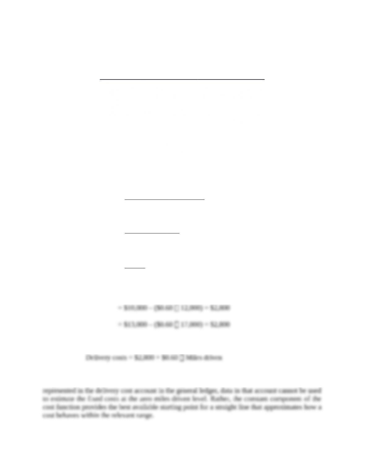
= $0.60 per mile
Constant = Total cost – (Slope coefficient Quantity of cost driver)
The cost function based on the two observations is
2. The cost function in requirement 1 is an estimate of how costs behave within the relevant
range, not at cost levels outside the relevant range. If there are no months with zero miles driven
10-7
10-22 Identifying variable-, fixed-, and mixed-cost functions. The Sunrise Corporation
operates car rental agencies at more than 20 airports. Customers can choose from one of three
contracts for car rentals of one day or less:
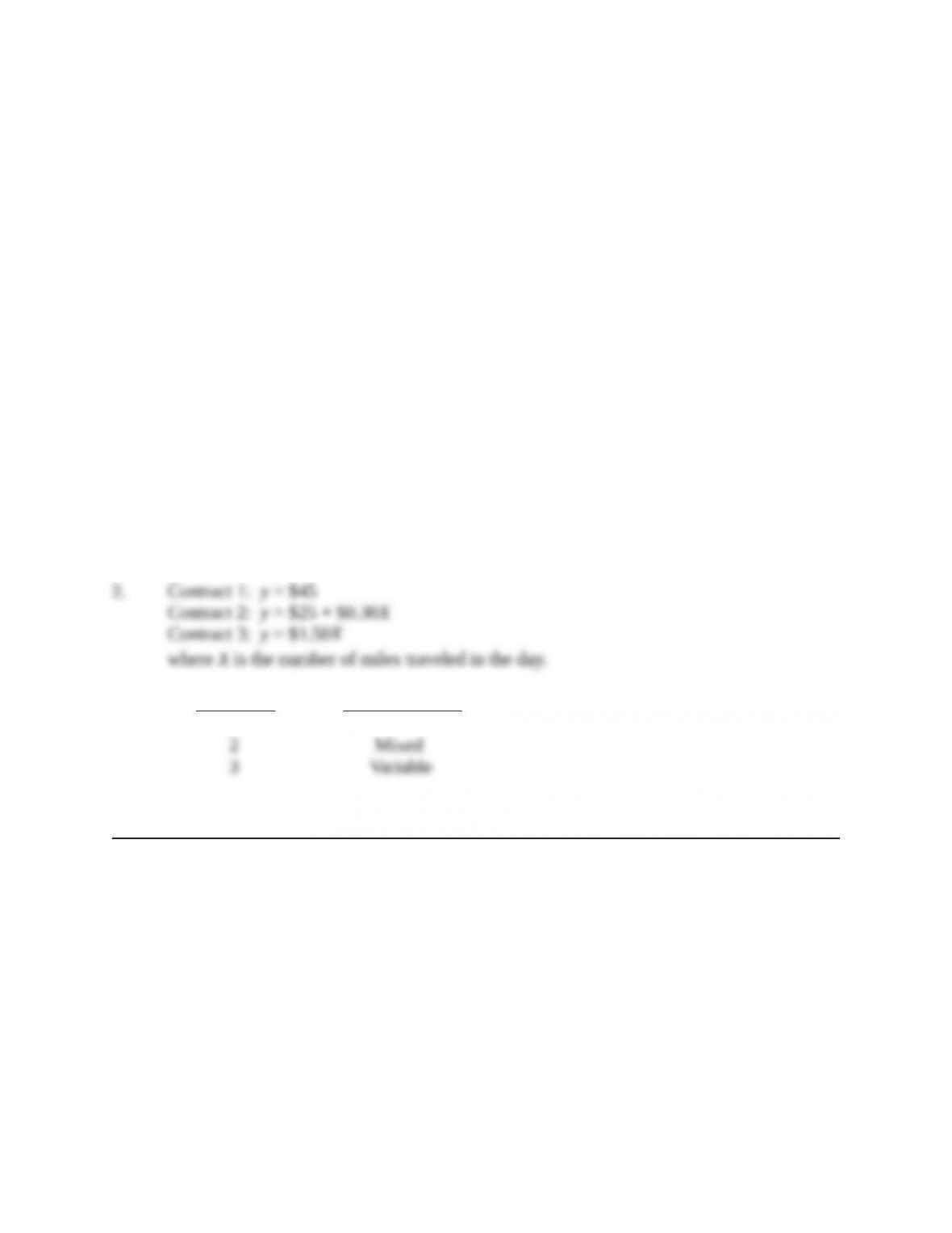
Contract 1: $45 for the day
Contract 2: $25 for the day plus $0.30 per mile traveled
Contract 3: $1.50 per mile traveled
Required:
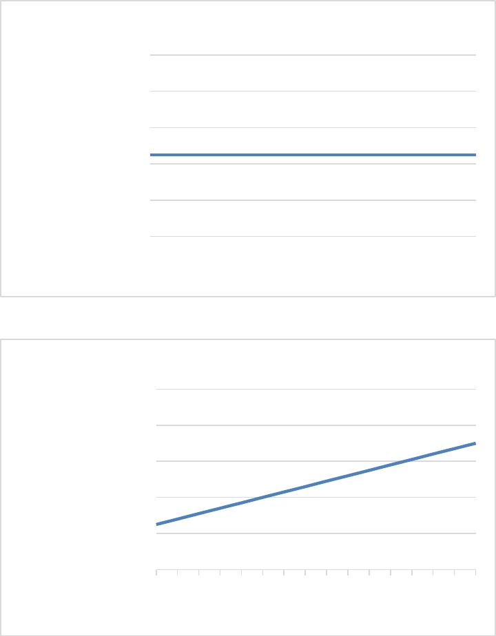
1. Plot separate graphs for each of the three contracts, with costs on the vertical axis and miles
traveled on the horizontal axis.
2. Express each contract as a linear cost function of the form
.y a bX= +
3. Identify each contract as a variable-, fixed-, or mixed-cost function.
SOLUTION
(15 min.) Identifying variable-, fixed-, and mixed-cost functions.
1. See Solution Exhibit 10-22.
3. Contract Cost Function
1
Fixed
SOLUTION EXHIBIT 10-22
Plots of Car Rental Contracts Offered by Sunrise Corp.
10-8
0 10 20 30 40 50 60 70 80 90 100 110 120 130 140 150
$0
$20
$40
$60
$80
$100
Contract 1: Fixed Costs
Miles Traveled Per Day
Car Rental Costs
….
..
…..
0 10 20 30 40 50 60 70 80 90 100 110 120 130 140 150
$0
$20
$40
$60
$80
$100
Contract 2: Mixed Costs
Miles Traveled Per Day
Car Rental Costs
….
10-9
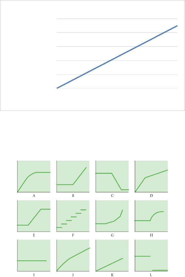
0 10 20 30 40 50 60 70 80 90 100 110 120 130 140 150
$0
$50
$100
$150
$200
$250
Contract 3: Variable Costs
Miles Traveled Per Day
Car Rental Costs
10-23 Various cost-behavior patterns. (CPA, adapted).
The vertical axes of the graphs below represent total cost, and the horizontal axes represent units
produced during a calendar year. In each case, the zero point of dollars and production is at the
intersection of the two axes.
Required:
Select the graph that matches the numbered manufacturing cost data (requirements 1–9). Indicate
by letter which graph best fits the situation or item described. The graphs may be used more than
once.
1. Annual depreciation of equipment, where the amount of depreciation charged is computed by
10-10
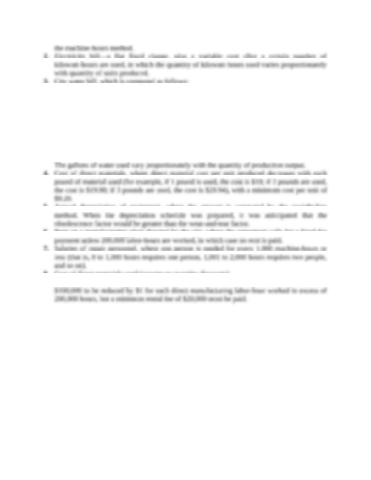
2. Electricity bill—a flat fixed charge, plus a variable cost after a certain number of
3. City water bill, which is computed as follows:
First 1,000,000 gallons or less $1,000 flat fee
Next 10,000 gallons $0.003 per gallon used
Next 10,000 gallons $0.006 per gallon used
Next 10,000 gallons $0.009 per gallon used
and so on and so on
4. Cost of direct materials, where direct material cost per unit produced decreases with each
5. Annual depreciation of equipment, where the amount is computed by the straight-line
6. Rent on a manufacturing plant donated by the city, where the agreement calls for a fixed-fee
7. Salaries of repair personnel, where one person is needed for every 1,000 machine-hours or
8. Cost of direct materials used (assume no quantity discounts).
9. Rent on a manufacturing plant donated by the county, where the agreement calls for rent of
10-11