Unlock document.
This document is partially blurred.
Unlock all pages and 1 million more documents.
Get Access
366 Copyright ©2017 Pearson Education, Inc.
3
O N L I N E T U T O R I A L
The Simplex Method of Linear Programming
DISCUSSION QUESTIONS
1. The fundamental purpose of the simplex procedure is to ena-
ble solutions to be found for sets of simultaneous equations in
which the number of variables exceeds the number of equations.
The simplex procedure is:
◼ Divide each value in the pivot row by the pivot number and
the pivot column except, cj, zj and cj – zj.
◼ Compute the zj as the sum of each column’s values multi-
cj – zj values are positive, you have an optimal solution.
Otherwise, return to first step.
2. Differences between graphical and simplex methods:
method is used); simplex checks a lesser number of
◼ Both find optimal solution at a corner point.
◼ Both require a feasible region and the same problem struc-
ture (objective function and constraints).
3. Pivot column:
◼ Select the variable column with the largest positive cj – zj
value (in a maximization problem) or largest negative cj – zj
value (in a minimization problem).
Pivot row:
4. In a maximization problem, the variable with the largest ob-
2.5, will enter first.
5. Slack variables are added only to “less than” constraints for
6. Steps in a simplex maximization problem:
◼ Step 1: Determine which variable enters the solution next.
◼ Step 2: Determine which variable to replace.
7. A surplus variable, used to convert “greater than” constraints
END-OF-TUTORIAL PROBLEMS
ONLINE TUTORIAL 3 THE SI M P L E X MET H OD OF LI N EA R PR O GR A M MI N G 367
Copyright ©2017 Pearson Education, Inc.
where:
x1 = number of coffee tables/week
x2 = number of bookcases/week
and then the system of equations entered into the simplex
cj
Solution Mix
9
12
0
0
Quantity
x1
x2
S1
S2
cj –
zj
9
12
0
0
x1
x2
S1
S2
0
S1
1/2
0
1
–1/2
4
12
x1
1/2
1
0
1/2
6
zj
6
12
0
6
72
cj
−
zj
3
0
0
–6
cj
Solution Mix
9
12
0
0
Quantity
x1
x2
S1
S2
9
x1
1
0
2
–1
8
Optimal: x1 = 8, x2 = 2, Profit = $96
T3.2 (a) The original equations are:
Objective: 3x1 + 9x2 (maximize)
Subject to: x1 + 4x2 24
x1 + 2x2 16
and then the system of equations entered into the sim-
plex tableau as shown below:
Initial simplex tableau:
cj
Solution Mix
3
9
0
0
Quantity
zj
0
0
0
0
0
cj –
zj
3
9
0
0
◼ Step 1: Identify the pivot column by finding the maximum
cj
−
zj
◼ Step 2: Identify the pivot row by dividing each value in the
◼ Step 3: Divide each value in the pivot row by the pivot
◼ Step 4: Multiply the new version of the pivot row by an-
other number in the pivot column (not the pivot number).
◼ Step 5: Compute the zj as the sum of each column’s values
(c) Second simplex tableau:
cj
Solution Mix
3
9
0
0
Quantity
x1
x2
S1
S2
0
S2
0.50
0
−
0.50
1
4
zj
2.25
9
2.25
0
54
cj
−
zj
0.75
0
−
2.25
0
x1
x2
S1
S2
9
x2
0
1
0.5
−
0.5
4
3
x1
1
0
−
1
2
8
zj
3
9
1.5
1.5
60
cj
−
zj
0
0
−
1.5
−
1.5
(e) In two iterations you should have the exact same results as
when starting from part (a) of this question. Your intermediate
tableau, however, will not relate to part (c) since you are solv-
(b)
368 ONLINE TUTORIAL 3 TH E SIM PL E X ME T H OD OF LI N EA R PR O G R AM M I N G
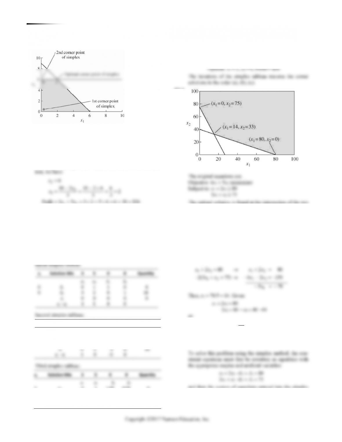
T3.3
The original equations are:
Objective: 3x1 + 5x2 (maximize)
Subject to: x2 6
3x1 + 2x2 18
x1, x2 0 (non-negativity)
The optimal solution is found at the intersection of the two
constraints. Solving for the values of x1 and x2 at the intersec-
Because this is a maximization problem, and the bottom
row of the tableau now includes only numbers that are
negative or zero, we have reached the optimal solution.
T3.4
ONLINE TUTORIAL 3 THE SI M P L E X MET H OD OF LI N EA R PR O GR A M MI N G 369
Initial simplex tableau:
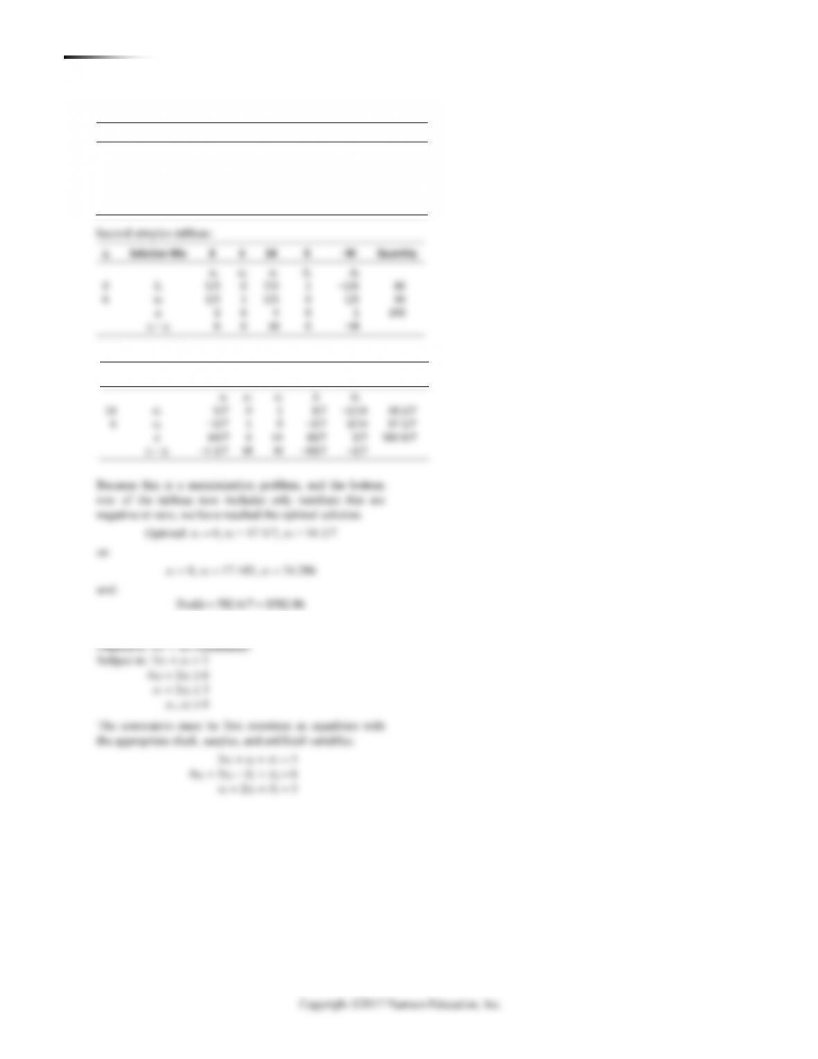
T3.5 Let x1 = number of class A containers to be used
Second simplex tableau:
cj
Solution Mix
4
5
0
0
M
M
Quantity
x1
x2
S1
S2
A1
A2
M
A1
0
1.67
–1
0.33
1
–0.33
55
4
x1
1
0.33
0
–0.33
0
0.33
25
zj
4
M
–M
M
M
–M
cj –
zj
0
–M
M
–M
0
M
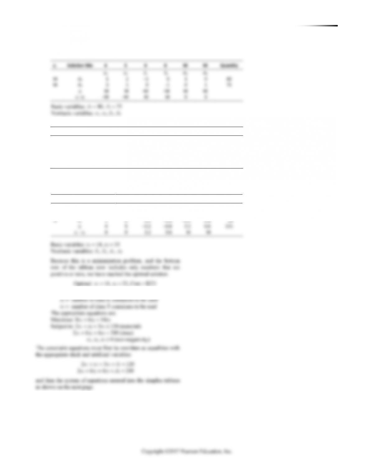
Basic variables: A1 = 55, x1 = 25
Nonbasic variables: x2, S1, S2, A2
Third simplex tableau:
cj
Solution Mix
4
5
0
0
M
M
Quantity
x1
x2
S1
S2
A1
A2
5
x2
0
1
–0.6
0.2
0.6
–0.2
33
370 ONLINE TUTORIAL 3 TH E SIM PL E X ME T H OD OF LI N EA R PR O G R AM M I N G
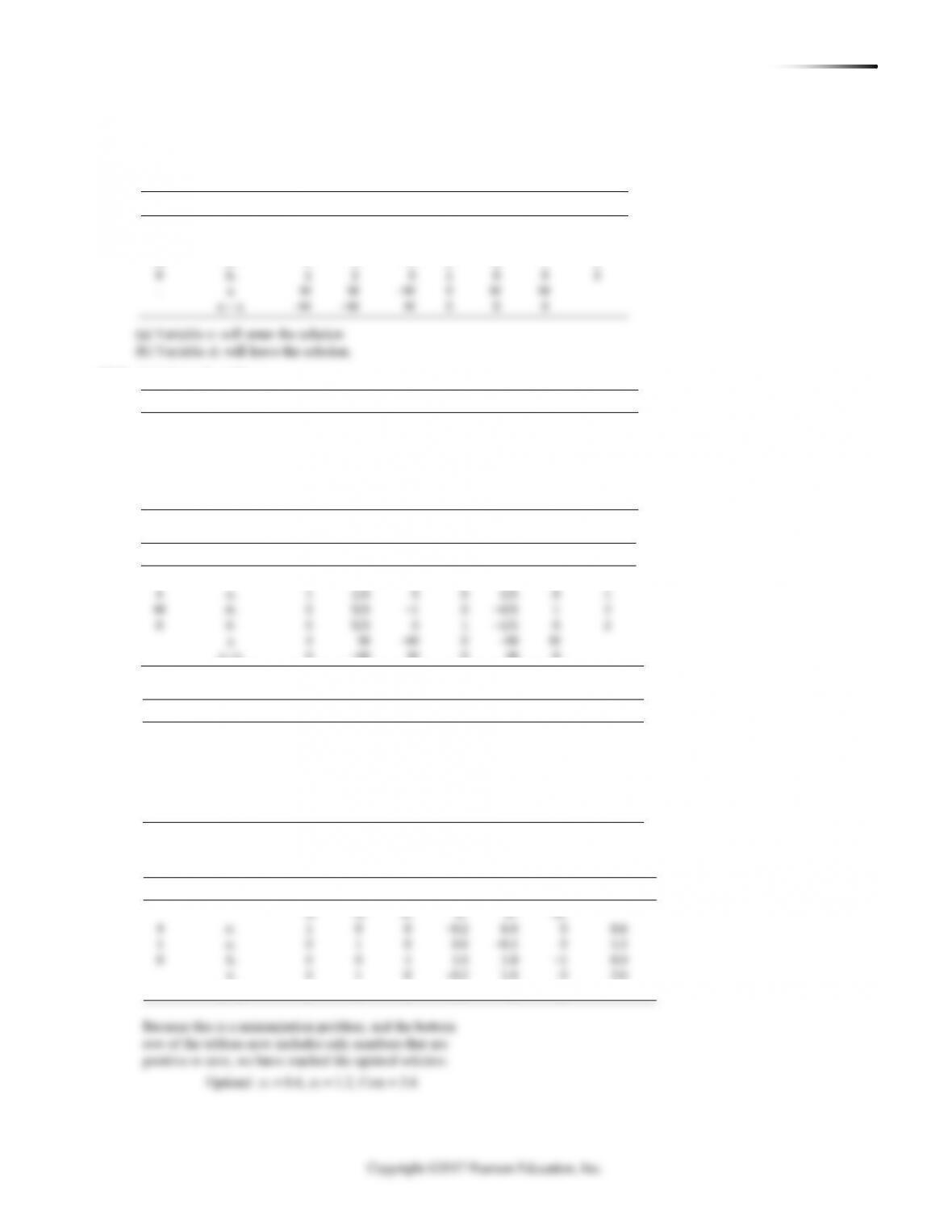
T3.6 The original equations are:
Initial simplex tableau:
cj
Solution Mix
8
6
14
0
–M
Quantity
x1
x2
x3
S1
A1
0
S1
2
1
3
1
0
120
–M
A1
2
6
4
0
1
240
zj
–M
–M
–M
0
–M
cj –zj
M
M
M
0
0
Third simplex tableau:
cj
Solution Mix
8
6
14
0
–M
Quantity
x1
x2
x3
S1
A1
ONLINE TUTORIAL 3 THE SI M P L E X MET H OD OF LI N EA R PR O GR A M MI N G 371
and then the system of equations entered into the simplex
tableau as shown below:
Initial simplex tableau:
cj
Solution Mix
4
1
0
0
M
M
Quantity
x1
x2
S1
S2
A1
A2
M
A1
3
1
0
0
1
0
3
M
A2
4
3
–1
0
0
1
6
T3.7
Initial simplex tableau:
cj
Solution Mix
4
1
0
0
M
M
Quantity
x1
x2
S1
S2
A1
A2
M
A1
3
1
0
0
1
0
3
0
S2
1
2
0
1
0
0
3
zj
M
M
–M
0
M
M
cj –
zJ
–M
–M
M
0
0
0
Second simplex tableau:
cj
Solution Mix
4
1
0
0
M
M
Quantity
x1
x2
S1
S2
A1
A2
4
x1
1
1/3
0
0
1/3
0
1
zj
4
M
–M
0
–M
M
cj –zj
0
–M
M
0
M
0
Third simplex tableau:
cj
Solution Mix
4
1
0
0
M
M
Quantity
x1
x2
S1
S2
A1
A2
4
x1
1
0
0.2
0
0.6
–0.2
0.6
1
x2
0
1
−0.6
0
–0.8
0.6
1.2
0
S2
0
0
1.0
1
1.0
–1.0
0.0
zj
4
1
0.2
0
1.6
–0.2
cj –
zj
0
0
–0.2
0
M
M
Note that this tableau is degenerate—the basic variable S2 has value 0.
Fourth simplex tableau:
cj
Solution Mix
4
1
0
0
M
M
Quantity


