352 BUSINESS ANALYTICS MODULE F SI M U LA T I O N
6
3
0.083
7
4
0.111
8
6
0.167
9
12
0.333
9
0.250
1
0.028
1
0.028
Lead
Cumulative
1
0.44
0.44
01–44
Time
Rand***
Demand
Place
Rand
Lead
1
14
07
6
6
8
0
Yes
60
2
2
8
77
10
8
0
2
No
—
—
3
0
49
9
0
14
9
No
—
—
6
0
16
7
0
0
7
No
—
—
7
0
14
7
0
0
7
No
—
—
13
14
39
9
9
5
0
Yes
73
2
14
5
89
10
5
0
5
No
—
—
15
0
88
10
0
14
10
No
—
—
16
14
24
8
8
6
0
Yes
01
1
17
6
11
7
6
14
1
No
—
—
23
14
75
10
4
0
Yes
33
1
24
4
95
11
4
14
7
No
—
—
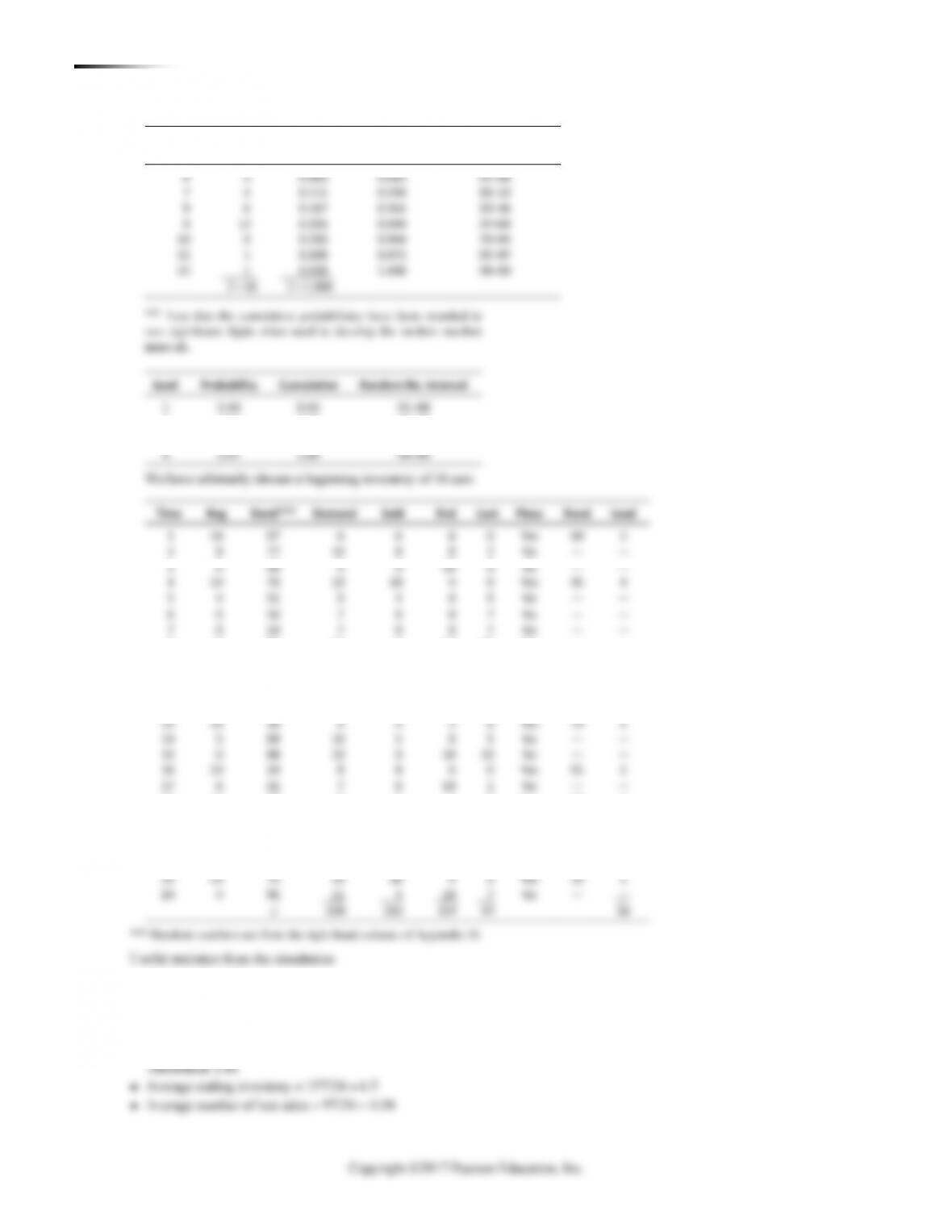
F.19 (a)
Demand for
Cumulative
Random Number
Mercedes
Freq.
Probability
Probability
Interval**
2
0.33
0.77
45–77
3
0.16
0.93
78–93
4
0.07
1.00
94–00
8
0
85
10
0
14
10
No
—
—
9
14
59
9
9
5
0
Yes
85
3
10
5
40
9
5
0
4
No
—
—
11
0
42
9
0
0
9
No
—
—
12
0
52
9
0
14
9
No
—
—
18
14
67
9
9
5
0
Yes
62
2
19
5
51
9
5
0
4
No
—
—
20
0
33
8
0
14
8
No
—
—
21
14
08
6
6
8
0
Yes
40
1
22
8
29
8
8
14
0
No
—
—
◼ Average demand
Simulation→209/24 = 8.71
Theoretical 8.75
◼ Average lead time
Simulation→16/8 = 2.00
Theoretical 1.86
Copyright ©2017 Pearson Education, Inc.
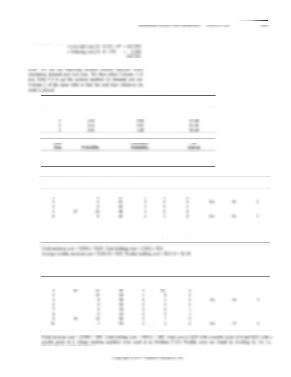
= $520,110, or $21,671 per month
2
0.20
0.80
61–80
3
0.15
0.95
81–95
Probability
The results are:
2
4
37
1
3
0
3
3
82
3
0
0
Yes
1
4
0
69
2
0
2
5
10
10
98
4
6
0
6
6
96
4
2
0
Yes
3
Week
Inv.
RN
Demand
Inv.
RN
4
10
69
2
8
0
5
8
98
4
4
0
Yes
63
3
6
4
96
4
0
0
7
0
33
1
0
1
8
0
50
1
0
1
9
10
10
88
3
7
0
10
7
90
3
4
0
Yes
57
3
Week
Units
Available
Begin
Inv.
RN
Demand
End
Inv.
Lost
Sales
Order?
RN
Lead
time
1
5
52
1
4
0
7
2
33
1
1
0
8
1
50
1
0
0
9
0
88
3
0
3
10
10
10
90
3
7
0
Total
23
5
F.21 If the reorder point in Problem F.20 is changed to 4 units, we have:
Units
Begin
End
Lost
Lead
1
5
52
1
4
0
Yes
6
1
2
4
37
1
3
0
3
10
13
82
3
10
0
Total
40
2
Total stockout cost = 2($40) = $80. Total holding cost = 40($1) = $40. Total cost is $120 with a reorder point of 4 and $223 with a
reorder point of 2. (Same random numbers were used as in Problem F.20.) Weekly costs are found by dividing by 10, i.e.,
$8 (stockout) and $4 (holding).
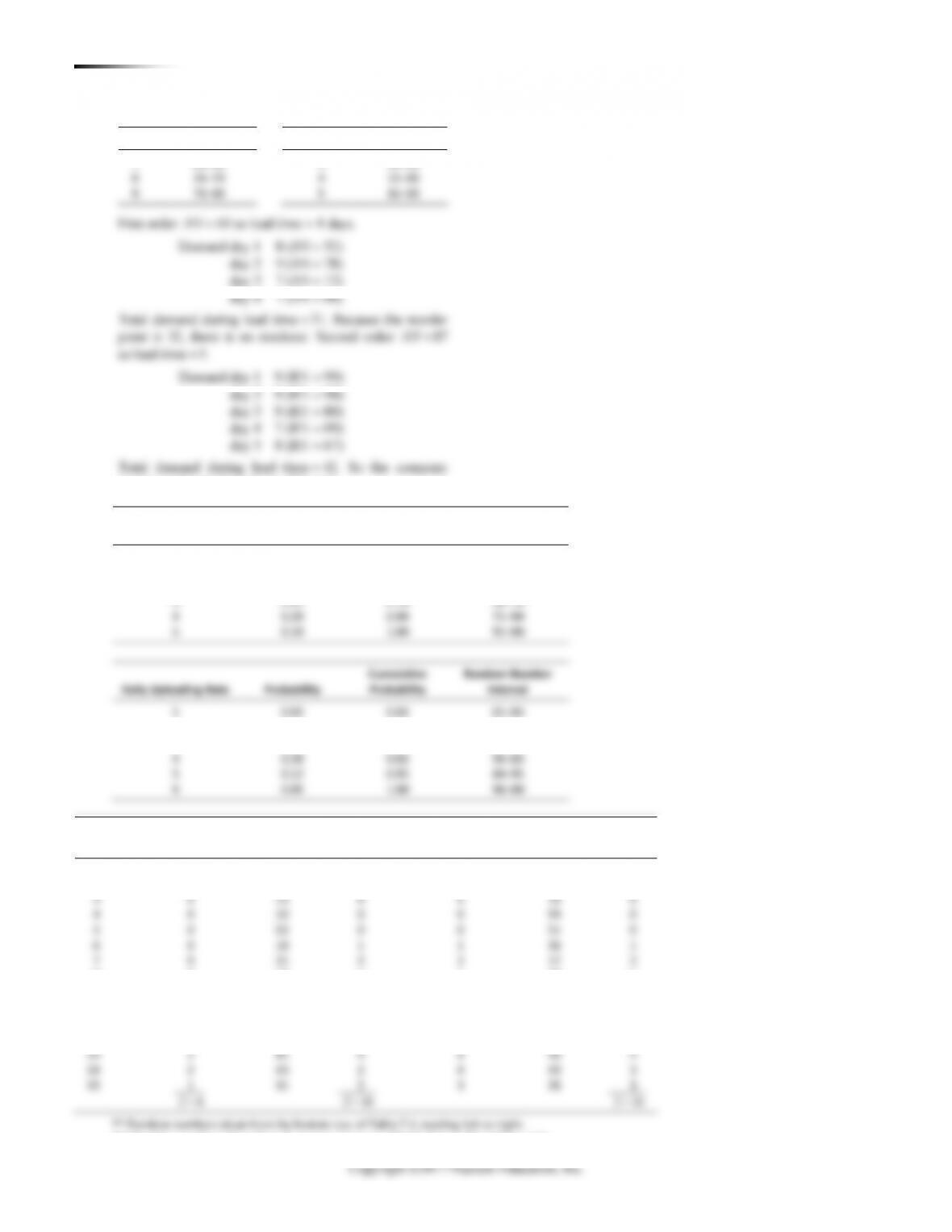
Demand
Probability
Cumulative
Probability
RN
Interval
0
0.20
0.20
01–20
1
0.40
0.60
21–60
4
0.05
1.00
96–00
Lead
Cumulative
RN
1
0.15
0.15
01–15
2
0.35
0.50
16–50
3
0.50
1.00
51–00
354 BUSINESS ANALYTICS MODULE F SI MU L A TI O N
F.22*
Sales
RN Interval
Lead Time
RN Interval
7
01–30
3
01–20
8
31–70
4
21–80
8 (RN = 52)
day 2
9 (RN = 78)
day 3
7 (RN = 13)
day 4
7 (RN = 06)
9 (RN = 99)
day 2
9 (RN = 98)
day 3
9 (RN = 80)
day 4
7 (RN = 09)
day 5
8 (RN = 67)
Total demand during lead time = 42. So the company
experienced a stockout during this time.
4
0.20
0.90
71–90
Cumulative
Random Number
Daily Uploading Rate
Probability
Probability
Interval
3
0.40
0.55
16–55
4
0.28
0.83
56–83
5
0.12
0.95
84–95
3
0
13
0
0
12
0
4
0
10
0
0
94
0
5
0
02
0
0
51
0
6
18
1
1
36
1
7
0
31
2
2
17
2
13
2
81
4
6
56
4
3
0.25
0.70
46–70
F.23*
Cumulative
Random Number
Number of Arrivals
Probability
Probability
Interval
0
0.13
0.13
01–13
1
0.17
0.30
14–30
2
0.15
0.45
31–45
2
0.12
0.15
04–15
Number
Daily
Total to be
Number
Day
Delayed
Random**
Arrivals
Unloaded
Random***
Unloaded
1
—
37
2
2
69
2
2
0
77
4
4
84
4
8
0
19
1
1
02
1
9
0
32
2
2
15
2
10
0
85
4
4
29
3
11
1
31
2
3
16
3
12
0
94
5
5
52
3
*** Random numbers taken from the next-to-last row of Table F.4, reading left-to-right.
BUSINESS ANALYTICS MODULE F SI M U LA T I O N 355
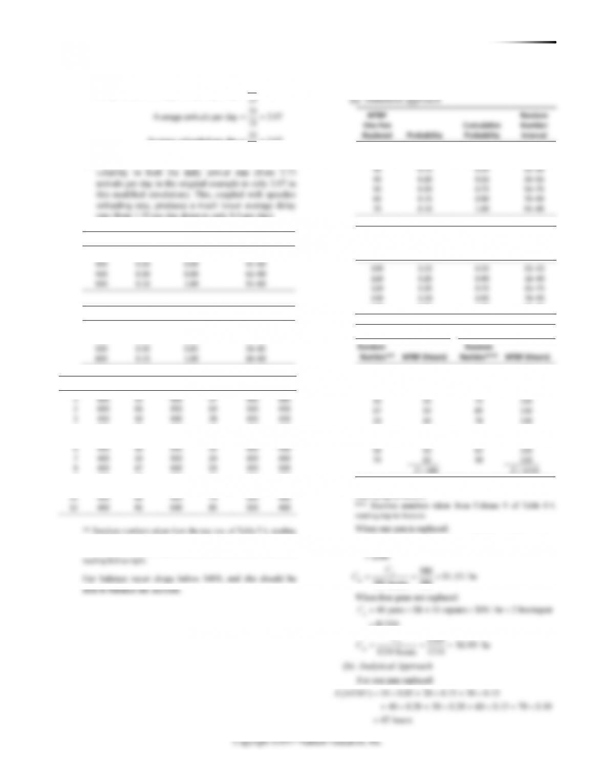
6
Average number of barges delayed per day 0.4
31
MTBF
Random
15
31
Average unloaded per day 2.07
15
==
==
(b) The short time span simulated (15 days) introduces
40
0.20
0.55
36–55
50
0.20
0.75
56–75
60
0.15
0.90
76–90
0.10
1.00
91–00
F.24*
Monthly
Probability
Cumulative
Random No. Interval
350
0.40
0.40
01–40
400
0.20
0.60
41–60
450
0.30
0.90
61–90
500
0.10
1.00
91–00
Monthly
Probability
Cumulative
Random No. Interval
300
0.10
0.10
01–10
400
0.45
0.55
11–55
500
0.30
0.85
56–85
600
0.15
1.00
86–00
11
450
66
450
74
500
400
F.25* MTBF = mean time between failures
One Pen
Cumulative
Number
Replaced
Probability
Probability
Interval
10
0.05
0.05
01–05
20
0.15
0.20
06–20
30
0.15
0.35
21–35
MTBF All
Random
Four Pens
Cumulative
Number
Replaced
Probability
Probability
Interval
100
0.15
0.15
01–15
110
0.25
0.40
16–40
120
0.35
0.75
41–75
130
0.20
0.95
76–95
140
0.05
1.00
96–00
One Pen Replaced
Four Pens Replaced
Random
Random
Number**
MTBF (Hours)
Number***
MTBF (Hours)
47
40
99
140
03
10
29
110
11
20
27
110
10
20
75
120
67
50
89
130
23
30
78
130
89
60
68
120
62
50
64
120
56
50
62
120
74
50
30
110
= 380
= 1210
** Random numbers taken from Column 8 of Table F.4,
( ) 10 0.05 20 0.15 30 0.15
40 0.20 50 0.20 60 0.15 70 0.10
42 hours
E MTBF = + +
+ + + +
=
Month
Beg
Rand**
Income
Rand***
Expense
End
1
600
52
400
37
400
600
2
600
06
350
63
500
450
3
450
50
400
28
400
450
4
600
88
450
02
300
600
5
500
53
400
74
500
500
6
450
30
350
35
400
450
7
400
10
350
24
400
400
8
400
47
400
03
300
500
9
500
99
500
29
400
600
10
600
37
350
60
500
450
Copyright ©2017 Pearson Education, Inc.
= $1.12/hour
Cost
Method
Replace One Pen
Replace Four Pens
Simulation
$1.53/hr
$1.09/hr
Analytical
$1.38/hr
$1.12/hr
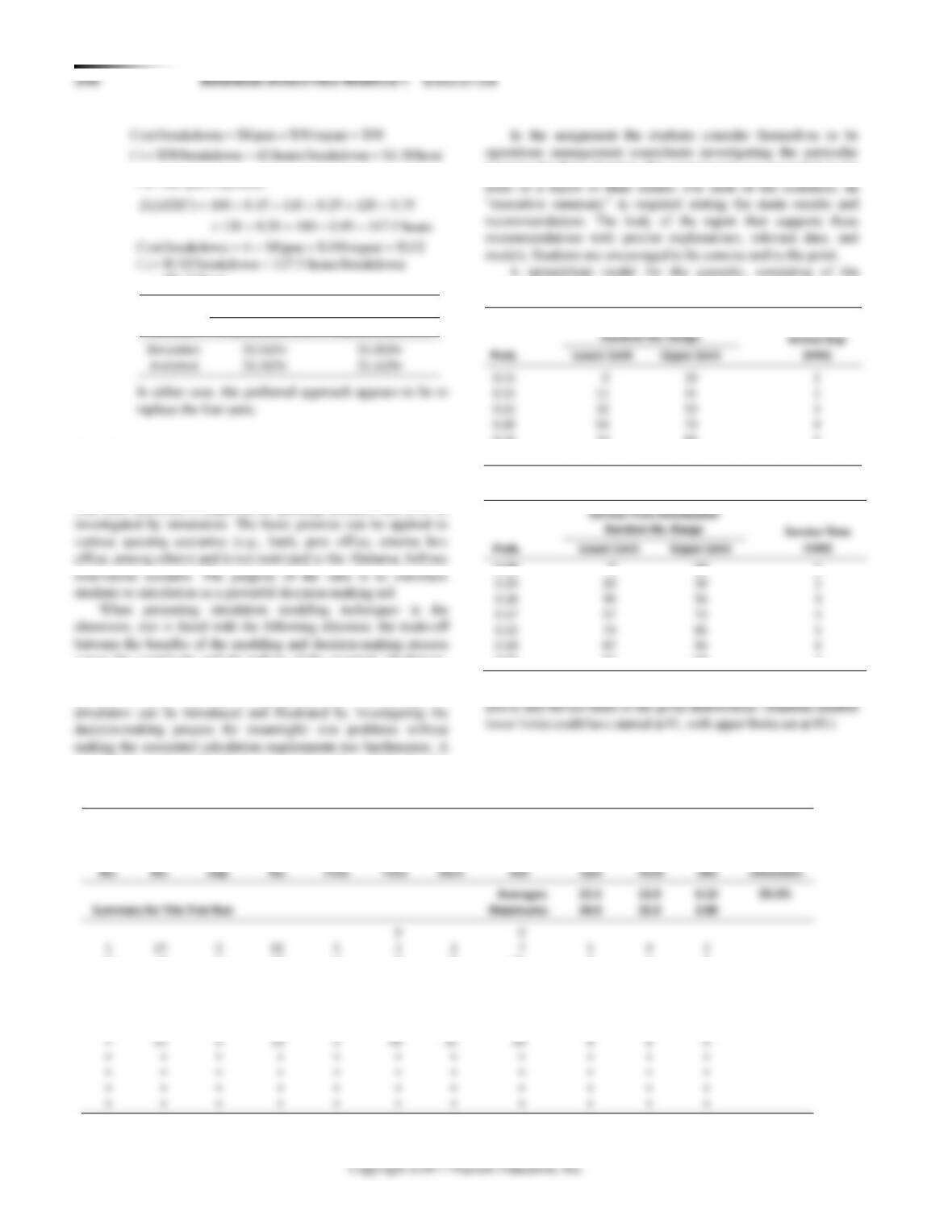
In either case, the preferred approach appears to be to
replace the four pens.
CASE STUDY
ALABAMA AIRLINES’ CALL CENTER
Service Time Distribution
Service Time
Prob.
Lower Limit
Upper Limit
versus the complexity and the tedium of the required calculations.
Spreadsheets that have a random number generator, such as Excel,
provide a means whereby the principles and methodology of
spreadsheet, such as Excel, is envisaged as the vehicle for this
simulation.
following items, should be constructed,
Arrival Interval Distribution
Random No. Range
Arrival Gap
(min)
Prob.
Lower Limit
Upper Limit
0.11
0
10
1
0.21
11
31
2
0.22
32
53
3
0.20
54
73
4
0.16
74
89
5
0.10
90
99
6
0.03
97
99
7
The two tables above are used for the random number generation of
Start
Hold
Averages:
15.5
12.0
Summary for This Trial Run
Maximums:
32.0
0
1
27
2
82
5
2
2
5
0
2
7
41
3
23
2
25
31
33
8
6
0
One Trial
Time
Time
Time
Cust
Rand
Arrival
Rand
Service
Arrival
Service
Service
in
on
Server
2
8
1
60
4
3
7
11
8
4
0
3
93
6
25
2
9
11
13
4
2
0
4
93
6
36
2
15
15
17
2
0
2
5
65
4
91
6
19
19
25
6
0
2
6
44
3
88
6
22
25
31
9
3
0
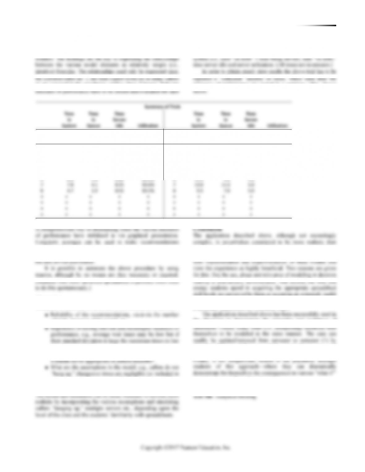
BUSINESS ANALYTICS MODULE F SI M U LA T I O N 357
The One Trial table (above) contains the actual model of the
as are required in the simulation window (here 2 hours). Relevant
Summary of Trials
Time
Time
Server
7
7.8
4.1
0.25
93.6%
7
13.0
11.0
5.0
8
4.7
1.9
0.55
83.5%
8
9.0
7.0
5.0
•
•
•
•
•
•
•
•
•
•
•
6
6.0
2.8
0.80
80.0%
6
14.0
9.0
4.0
regarding hiring a second reservation agent.
For part (b) essentially the above approach is repeated with
Discussion
of trials, structure of the model, etc.
may be unacceptable.
◼ Labor standard issues: is a utilization of e.g., 95 percent for
service times), there are no calls in the system at “time
zero” etc. What are the implications/restrictions?
trial—here, for example, the average and maximum of time in
measures of performance are stored in a summary table, shown
could normally be attempted without resorting to a simulation
model. Even the least “quantitatively oriented” students persevere
skill, as an in-depth familiarity with a spreadsheet package is now
the classroom to demonstrate the principles and usefulness of
changing Alabama Airlines to a bank, movie theater, etc., and
(2) by changing the arrival interval and service time distributions.
scenarios by amending a few parameters.
LO F.4: Use Excel spreadsheets to create a simulation
System
Queue
Idle
Utilization
System
Queue
Idle
Utilization
Avg:
8.9
5.7
0.40
88.4%
Max:
18.0
14.5
4.3
98.1%
Trial #
Trial #
1
7.6
4.0
0.43
89.5%
1
14.0
10.0
4.0
2
8.6
5.1
0.23
93.9%
2
17.0
15.0
5.0
3
3.8
1.2
1.00
72.4%
3
10.0
7.0
5.0
4
17.3
13.8
0.25
93.4%
4
30.0
27.0
3.0
5
4.8
1.8
0.65
82.3%
5
11.0
6.0
6.0
358 BUSINESS ANALYTICS MODULE F SI MU L A TI O N
ADDITIONAL CASE STUDY (AVAILABLE IN MYOMLAB)
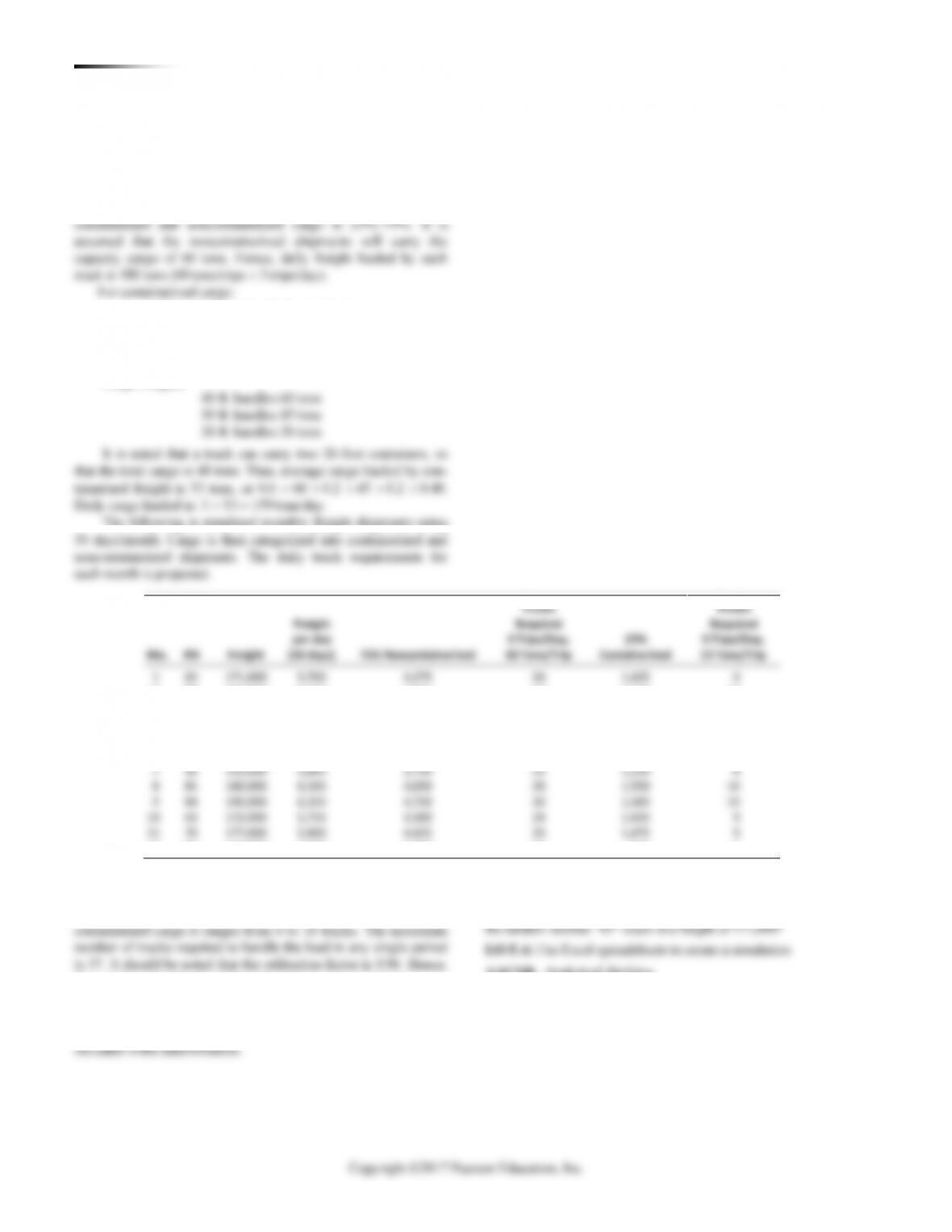
SAIGON TRANSPORT
The table in the case represents a cumulative normal distribution
of monthly cargo tonnages. The distribution of cargo between
60% is packaged in 40-ft. containers
20% is packaged in 30-ft. containers
20% is packaged in 20-ft. containers
1
63
171,000
5,700
4,275
24
1,425
9
7
36
150,000
5,000
3,750
21
1,250
8
8
81
186,000
6,200
4,650
26
1,550
10
9
84
190,000
6,333
4,750
26
1,583
10
10
63
172,000
5,733
4,300
24
1,433
9
11
70
177,000
5,900
4,425
25
1,475
9
As seen from the simulated year’s operation, the daily truck
requirement for noncontainerized cargo ranges from 15 to 27. For
the number of trucks should be adjusted upward accordingly.
Students should simulate future periods with a given fleet
size weighing the opportunity cost of trucks (cost of capital)
against demurrage penalties. Container demurrage should also be
A discussion of obtaining a simulated “Freight” from a
“Random Number” should be highlighted; for example, why does
Trucks
Trucks
2
88
197,000
6,567
4,925
27
1,642
10
3
55
165,000
5,500
4,125
23
1,375
9
4
69
176,000
5,867
4,400
24
1,467
9
5
13
124,000
4,133
3,100
17
1,033
7
6
17
131,000
4,367
3,275
18
1,092
7
12
06
110,000
3,667
2,750
15
917
6