D
B U S I N E S S A N A L Y T I C S MOD U L E
Waiting-Line Models
DISCUSSION QUESTIONS
1. Three parts of a queuing system: arrivals or inputs to the
LO D.1: Describe the characteristics of arrivals, waiting lines, and
service systems
2. Qualitative concerns include fairness and the aesthetics of the
area in which waiting takes place.
schedule or randomly); and the behavior of the arrivals (joining
4. Measures of system performance:
◼ The average queue length;
◼ The probability of a specific number of customers or objects
5. Service times occur according to the negative exponential
distribution.
6. The service rate is faster than the arrival rate.
6. This is, of course, how most supermarket bakeries operate—
FCFS by the use of numbers. This is good because at the bakery,
we cannot distinguish long jobs from short ones. (This can be
compared with the situation at the checkout counter; where we
7. “Balk” is to refuse to enter the queue: “renege” is to leave the
service systems
8. Ws is the time spent waiting plus being serviced, Wq is the
of when other rules are more appropriate include:
326 BUSINESS ANALYTICS MODULE D WA I T I N G – L I N E MO D E L S
10. If : Intuitively, the queue will grow progressively
longer, because the arrival rate is larger than the service rate.
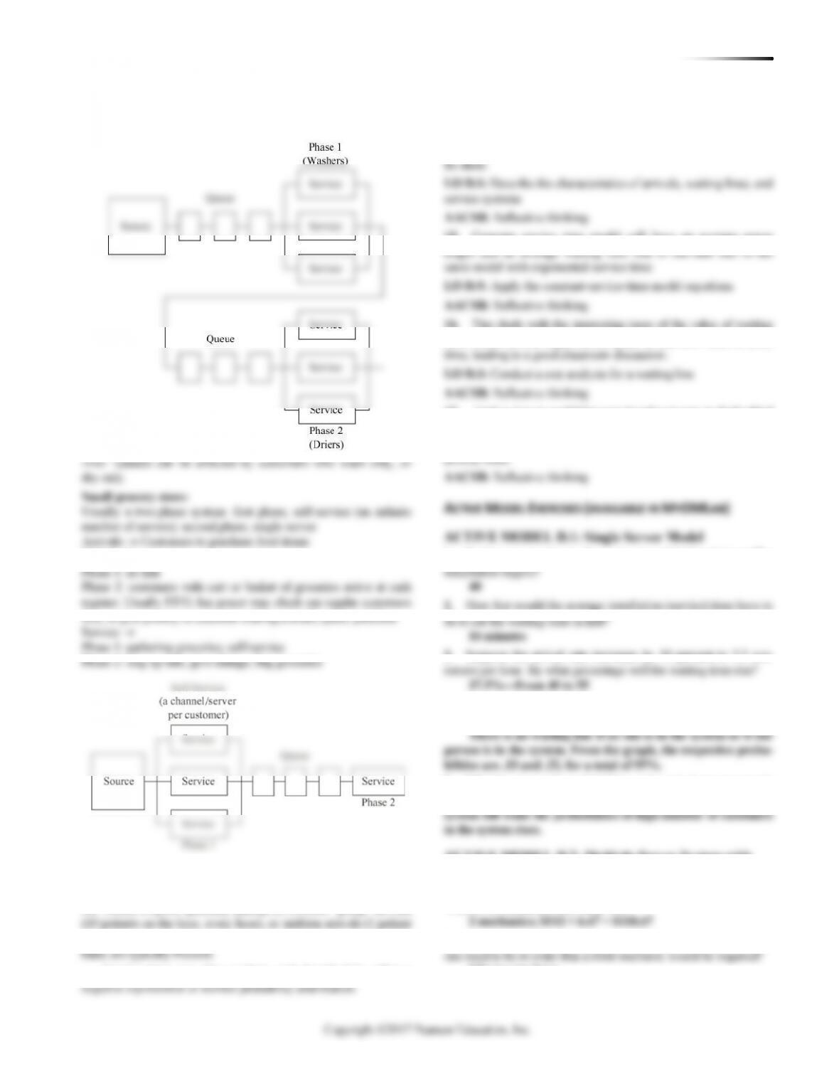
13. Barber shop:
Arrivals → Customers wanting haircuts
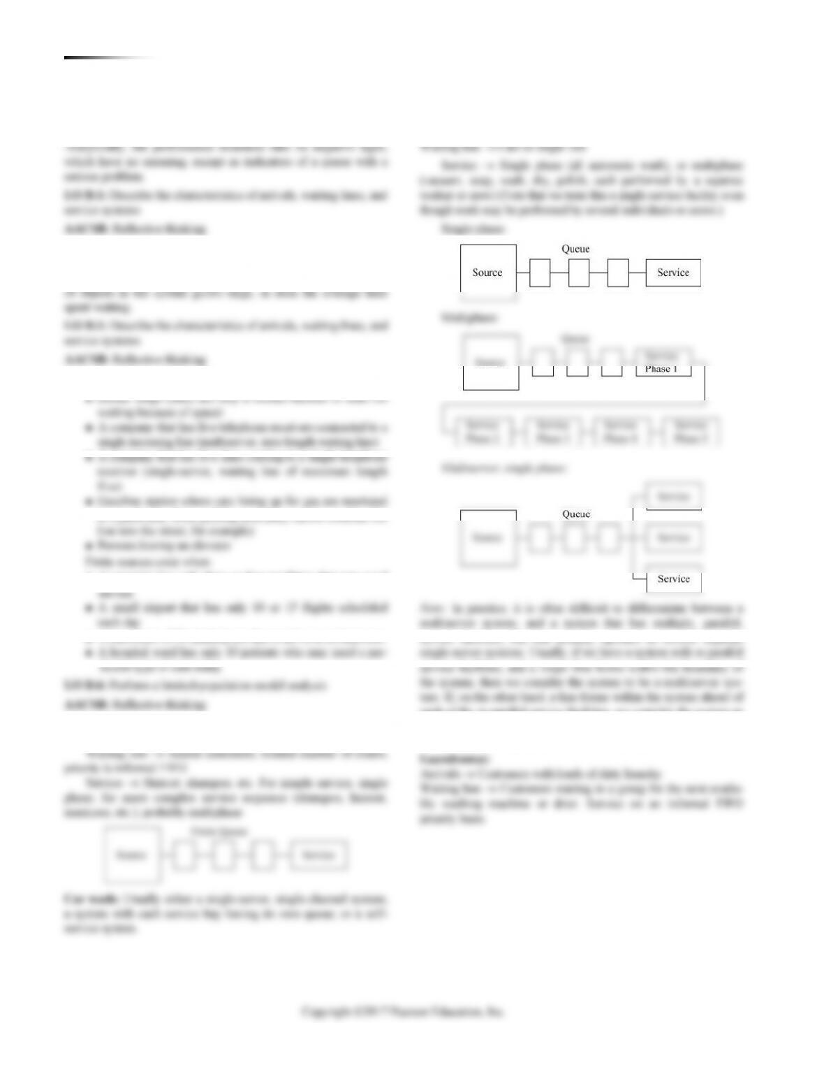
Single server:
Arrivals → Dirty cars
each of the m parallel service facilities, we consider the system as
if it were m separate single-server systems, each with an arrival
rate equal to the original arrival rate divided by m.
BUSINESS ANALYTICS MODULE D WA I T I N G – L I N E MO D E L S 327
Service facility → Two–phase system (washer, drier); each phase
multiserver.
Waiting line →
LO D.4: Apply the multiple-server queuing model formulas
AACSB: Application of knowledge
every 15 minutes). Arrivals at an emergency center, on the other
Service times are often random, and described by either a
Service times would approach a constant only when the physi-
cian provided approximately the same treatment to each patient.
This might occur in the case of physical exams, or a clinic providing
15. Constant service time model will have an average queue
time. Some service organizations place a very low value on your
17. Little’s Law is useful because it makes it easy to find a third
parameter if two are already computed/known. The law makes no
assumptions about probability distributions, number of servers, or
1. For how many minutes do customers wait before their muffler
4. What is the probability that there is no waiting line when a
car arrives for service?
5. What happens to the probabilities as the arrival rate increases?
The probabilities of low numbers of customers in the
ACTIVE MODEL D.2: Multiple Server System with
Costs
1. What number of mechanics yields the lowest total daily cost?
2. Use the scrollbar on the arrival rate. What would the arrival
3.8 cars per hour
BUSINESS ANALYTICS MODULE D WA I T I N G – L I N E MO D E L S 329
k
+
=
k
P
1
0
0.667
1
0.444
2
0.296
3
0.198
D.5
D.4
==
=
−
−
2
100 200
/ /1 where: 20 / hour, 10 / hour
(b) = = 0.5
(d) = = = 0.5
()
(e) = = 0.05 hours
q
s
MM
L
W
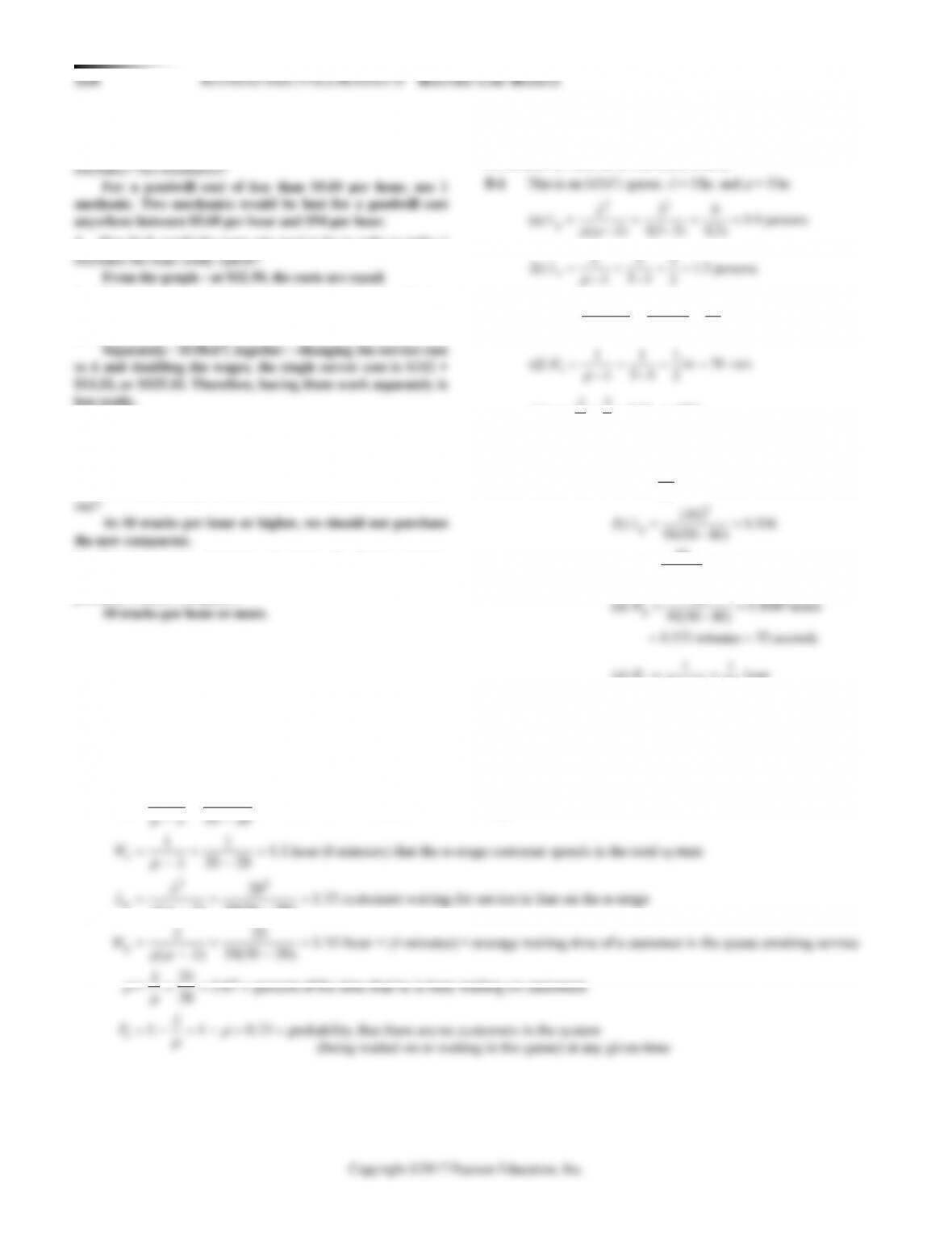
M/M/1 model:
= 12,
= 15
So Lq = 3.2
(b) Wq = Average time a prescription spends in the queue:
12
= = =
.1523
Then .0127 hr. = .76 minutes 46 sec.
12
q
W= =
D.6
= = = =
−−
= = =
−−
==
++
==
= = −
( ) ( )
−−
= = =
−−
+
= = =
180/hour, 120/hour,
/ /1 model with
or 3/min. and 2/min.
MM
==
==
D.7 This is an M/M/1 model. = 24,
= 30
0
30 24 6
( ) 30(30 24) 30(6)
24 24 2
( ) 30(30 24) 30(6) 15
1
(e) 1 / 1 24 / 30 .20
5
24
s
q
P
−−
−−
−−
= − = − = =
4.80
24 24
.640 .512 0.128
30 30
= − = − =
D.8 M/M/1 model with
= 3,
= 8
(a) The utilization rate,
, is given by:
(b) The average down time, Ws, is the time the machine
waits to be serviced plus the time taken to perform the
service.
11
(c) The number of machines waiting to be served, Lq, is, on average:
22
30.225 machines waiting
q
L
= = =
(d) Probability that more than one machine is in the system:
39
Probability that more than 2, 3, or 4 machines are in the system:
3
4
8 512
330 BUSINESS ANALYTICS MODULE D WA I T I N G – L I N E MO D E L S
(e) The probability that there are more than two people in
D.9 This is an M/M/1 model; = 10,
= 15
BUSINESS ANALYTICS MODULE D WA I T I N G – L I N E MO D E L S 331
(d) The probability that there are more than three trucks in
the system, Pn > 3, is given by:
1
4
3
30 0.540
35
k
nk
n
P
P
+
=
==
Thus, the probability that there are more than three
trucks in the system is 0.540.
To determine total cost using the second clerk (a second server):
01
11
!!
0
0 1 2 2 15
1 12 1 12 1 12
0! 15 1 15 1 2 15 2 15 12
1
1
1
nM nM
M
n M M
n
P
=−
−
=
−
=
+
=
++
332 BUSINESS ANALYTICS MODULE D WA I T I N G – L I N E MO D E L S
Therefore, the optimum number of clerks is 2.
D.14
= 15/hour,
= 20/hour
Wq = 0.0083 hours =
1
2
minute = 30 sec.
Lq = 0.083 people
and 2 as exits.
(b) The students should recognize and question all the lim-
independent and Poisson. But are exiting passengers
independent? More realistically, they arrive in batches
(as a train arrives), and unless trains unload every
minute or two, this assumption may be unreasonable.