CHAPTER 9
PRICING AND OUTPUT DECISIONS:
MONOPOLISTIC COMPETITION AND OLIGOPOLY
QUESTIONS
1. The key difference is “product differentiation.”
2. a. In a pure monopoly, no one else can enter the market. Thus, the monopolist will enjoy
(Instructors may wish to discuss how realistic this is in the real world, i.e., how feasible is it for
any non-regulated company to enjoy a monopoly over a long period of time.)
b. Oligopolists may enjoy above-normal profits as long as their dominance in the market
c. Because of the ease of entry in this market, we expect any above-normal profits to eventually
d. Because of ease of entry into the market, any above-normal profits (economic profits) will
3. Perhaps one of the most publicized examples of this is the bank credit card. In effect, the funds
4. Students should agree with this statement. A profit-maximizing firm will set a price according to the
“MR=MC” rule. Firms that wish to maximize market share will.ry to increase their revenue. Thus,
5. One of the main reasons why firms might not be able to set a price according to this rule is the
difficulty and/or cost of obtaining the data on MR and MC. Indeed, firms might have to consider
Copyright © 2014 Pearson Education, Inc.
Pricing and Output Decisions: Monopolistic Competition and Oligopoly90
6. Interdependence in a market means that each firm sets a price with the explicit consideration of the
reactions of its competitor. Thus, in this situation, it is possible that all firms would continue to
7. A price leader provides a mechanism for everyone to begin raising prices in a more orderly and
8. The usual concentration ratios could be used. Also, pricing tactics of competitors could be traced to
9. a. Oligopoly in the national (or worldwide) fast food market, but monopolistic competition in
b. Oligopoly in the national (or worldwide) oil refinery market; monopolistic competition at the
c. Monopolistic competition. The top five computer manufacturers (Dell, Compaq, IBM,
d. Oligopoly (almost a duopoly if you think about Heinz and Del Monte essentially dominating
e. Oligopoly (main competitor to Procter’s “Pampers” is Kimberly-Clark’s “Huggies”). However,
f. Oligopoly (there is, of course, the green box, and private store labels are also increasing in
g. Monopolistic competition. Starbucks may be alone as a national chain, but in local markets
h. Oligopoly in national pizza chains. Monopolistic competition at the local level.
i. Oligopoly, but because of Intel’s dominance in this market, it could be called “near monopoly.”
10. The S-C-P paradigm says that industry structure determines industry conduct, which in turn
Copyright © 2014 Pearson Education, Inc.
Pricing and Output Decisions: Monopolistic Competition and Oligopoly91
11. (1) Threat of new entrants: relates to number of sellers in perfect and monopolistic competition.
12. a. The beer industry in the United States is already oligopolistic. One of the main reasons why
As far as world markets are concerned, this may put SAB into genuine contention with
Heineken and Interbrew, the two brewery giants mentioned in the chapter.
b. As mentioned above, one of SAB’s main reasons for buying Miller is to gain direct access to
Looking at the deal from Philip Morris’ point of view, Miller’s sales made up less than 5% of
Copyright © 2014 Pearson Education, Inc.

Pricing and Output Decisions: Monopolistic Competition and Oligopoly92
PROBLEMS
1. a. Note to Instructors: We found this problem to be a good application of the concepts. We also
found that this makes a good in-class assignment. If your class size allows for this, divide the
class into groups of 4 to 6 students and have each be prepared to report to the class their
recommendation.
Please be aware that students may not realize at first that this problem assumes a constant MC
(which therefore equals AVC). You may wish to provide this hint. However, it is interesting to
let the students discover on their own about the nature of a linear total cost function.
It is interesting to note the different approaches that students use to solve this problem. Some
use the more cumbersome “TR/TC Approach,” while others go right to the marginal analysis
and begin comparing MR with (the constant) MC or AVC.
PRPWQ TR MR E
12.50 10.00 6,000 60,000
12.00 9.60 6,500 62,400 4.80 -1.96
11.50 9.20 7,000 64,400 4.00 -1.74
11.00 8.80 7,500 66,000 3.20 -1.55
10.50 8.40 8,000 67,200 2.40 -1.38
10.00 8.00 8,500 68,000 1.60 -1.24
9.50 7.60 9,000 68,400 0.80 -1.11
9.00 7.20 9,500 68,400 0.00 -1.00
8.50 6.80 10,000 68,000 -0.80 -0.90
8.00 6.40 10,500 67,200 -1.60 -0.80
b. $8.75 is definitely a “sub-optimal” price as far as the students are concerned, because at that
price MR < MC. In fact, this price actually falls in the inelastic portion of the demand curve.
Thus, it would not even yield maximum total revenue.
(The elasticity of demand between $12.50 and $8.00 is -1.24, indicating that demand is elastic
over this price range. However, dividing up this range into smaller intervals of $.50 reveals that
$8.75 actually falls in the inelastic position of the demand curve.)
In order to determine the profit maximizing price, we must first determine the firm’s marginal
cost of production. We shall assume the following costs to be variable:
Paper $12,000
Repro Services 8,000
Binding 3,000
Shipping 2 ,000
Total Variable Cost $25,000 (Total fixed cost = $20,000)
AVC = $4.16. Because it is constant, we can also state that it is equal to MC.
Based on the demand schedule above, an MC of $4.16 would fall somewhere between the retail
price of $12.00 and 11.50.
Copyright © 2014 Pearson Education, Inc.
Pricing and Output Decisions: Monopolistic Competition and Oligopoly93
c. Let us assume that the retail price is set at $12.00 (a nice round number). At this level, total cost
would be $47,040 (TFC = $20,000 and TVC = $4.16 x 6500). Total profit would be $15,360.
Although this venture looks profitable, it does not seem to provide the students with economic
profit. In fact, from an economic standpoint, each student would incur a loss because each
student’s assumed share in the profits of $3072 is not enough to cover the assumed opportunity
cost of $4000. Unless the students want the experience of running their own business, the
“economics” of this venture dictate that they not start this company.
d. Given the bookstore’s costs (which we do not know), $8.75 may very well be its optimal price.
Moreover, the store manager may want to consider the book as a “loss leader” or at least an
item whose low price might attract customers into the store.
2. a. The main difference is that the inclusion or exclusion of miscellaneous cost affects the MC,
thereby affecting the point at which MC = MR. When miscellaneous cost is considered to be
variable, MC = $5.00. The optimal price would be about $12.75. When it is not included, MC =
$4.16. Thus, the optimal price would be about $11.75.
b. In this problem, it is not likely that the law of diminishing returns would be important.
However, AVC and MC could rise if for some reason factor costs rose (e.g., increase in wage
rates of printers due to overtime compensation).
c. AVC and MC would probably not decrease in the short run. In the long run, they might if the
students increase their operations and cut costs from economies of scale (e.g., printing and
paper costs are reduced if the printer cuts the price because of higher production runs).
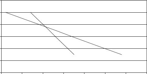
3. a. and b.
Firm’s Demand Curve Industry Demand Curve
Price Quantity
Total
Revenue
Margina
l
Revenue
Price Quantity
Total
Revenue
Margina
l
Revenue
10.00 2 20 10.00 14 140
9.00 10 90 8.75 9.00 17 153 4.33
8.00 18 144 6.75 8.00 20 160 2.33
7.00 26 182 4.75 7.00 23 161 0.33
6.00 34 204 2.75 6.00 26 156 -1.67
5.00 42 210 0.75 5.00 29 145 -3.67
4.00 50 200 -1.25 4.00 32 128 -5.67
3.00 58 174 -3.25 3.00 35 105 -7.67
Copyright © 2014 Pearson Education, Inc.
D Ind.
D Firm
0
2
4
6
8
10
12
0 10 20 30 40 50 60 70
Q
P
Pricing and Output Decisions: Monopolistic Competition and Oligopoly94
Figure 9.1
Copyright © 2014 Pearson Education, Inc.
Pricing and Output Decisions: Monopolistic Competition and Oligopoly95
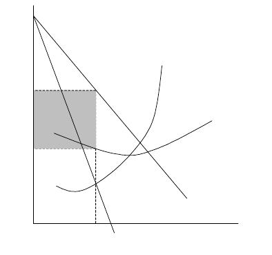
c., d., e.
Figure 9.2
The range of changes in marginal costs without impact on price is shown on above graph. It is
the vertical distance between the two marginal cost curves vertically below the kink.
4. a. FALSE Not if its loss is less than its fixed cost. See explanation of problem 1.
b. FALSE Even a pure monopoly has to consider the possibility of demand falling below
the level sufficient to earn a profit. (For example, even if Polaroid continues to
have a monopoly on cameras that use instant developing film, can they stop the
erosion in demand due to the one-hour photo developing machines and cameras
that record images electronically on discs?)
c. TRUE Other factors held constant, the entry or exit of firms will theoretically lead to
this condition.
d. TRUE In order to maximize revenue, a firm will price its product at the point where
MR=0. By implication, this must be a lower price than the point where MR=MC.
e. FALSE Although this is often the case, it is not always so.
f. TRUE Economists consider this to be true because the more opportunities for
substitution that a consumer has, the more elastic the demand for a particular
product tends to be. In a monopolistically competitive market, there are many
more firms for consumers to choose from.
5. a. Their unit cost of goods sold might be lower because they could buy directly from the
manufacturer. Also, if consumers are not brand-loyal, stores might be able to increase revenues
by lowering price. Thus, private label products could be (and often are) more profitable to sell
than national brands.
b. Selling to stores could help to reduce excess capacity. If they then produce at maximum
capacity, their unit costs would be minimized.
6. a. Regardless of their cost structure, all three would be earning less money because the demand is
price inelastic over this range of prices.
Copyright © 2014 Pearson Education, Inc.
MR
D
0
2
4
6
8
10
12
0 10 20 30 40 50 60 70
Q
P
Pricing and Output Decisions: Monopolistic Competition and Oligopoly96
b.Perhaps, depending on their respective marginal costs.
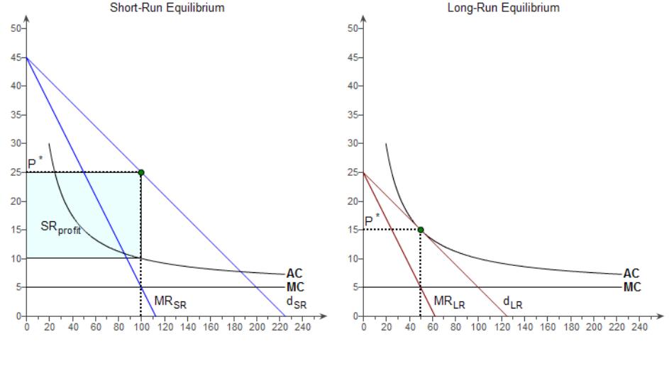
7. a. P= $25 and the firm is earning a short-run positive economic profit.
b. As new competitors enter the market, economic profit would decrease, eventually reaching
zero.
c. In the long run, the firm will lower its price to $15, reduce output, and will earn zero economic
profit.
d. In the long run, the firm’s demand curve will rotate inward, the price doesn’t change, but the
equilibrium quantity decreases.
Copyright © 2014 Pearson Education, Inc.
Pricing and Output Decisions: Monopolistic Competition and Oligopoly97
e. The demand in part d represents a decrease in market share for the representative firm.
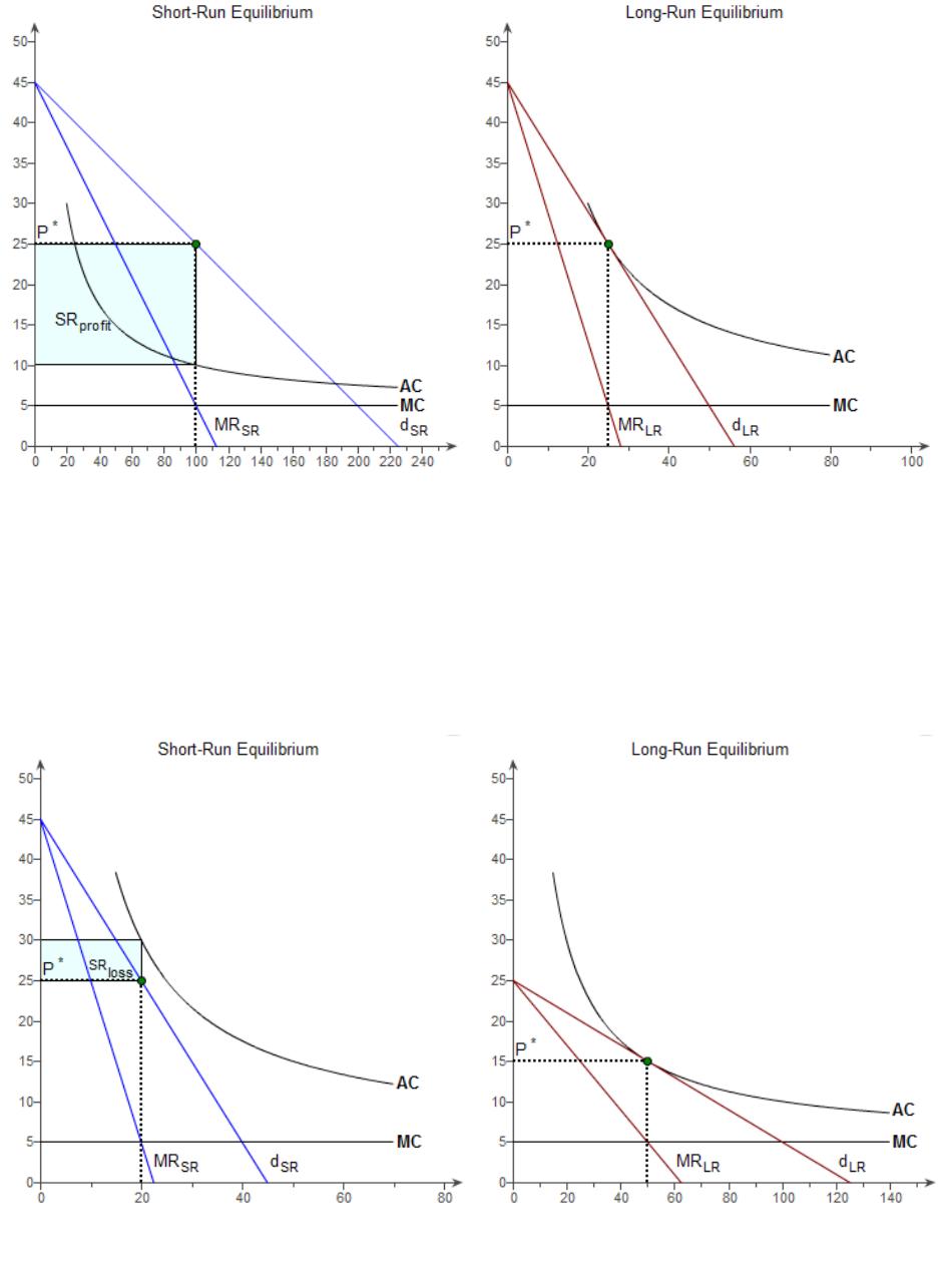
8. a. P= $25 and the firm is earning a short-run economic loss.
b. As firms exit the market, economic losses will decrease, eventually reaching zero.
c. In the long run, the firm will lower its price to $15, increase output, and will earn zero
economic profit.
Copyright © 2014 Pearson Education, Inc.
Pricing and Output Decisions: Monopolistic Competition and Oligopoly98
d. In the long run, the firm’s demand curve will rotate outward, the price doesn’t change, but
the equilibrium quantity increases.
e. The demand in part d represents anincrease in market share for the representative firm.
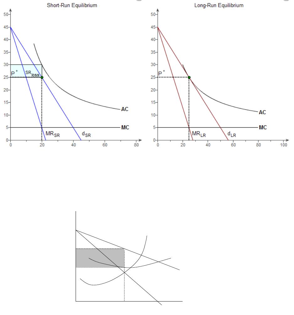
9. “Low-Cost Approach”
Figure 9.3
Monopolistic competitor is able to keep AC low enough so that it is able to earn an economic profit
given its demand.
“Differentiation Approach”
Copyright © 2014 Pearson Education, Inc.
Q
MR
D
AC
MC
P
P
1
Q
1
Pricing and Output Decisions: Monopolistic Competition and Oligopoly99
Figure 9.4
Differentiation causes D to become less elastic, thereby enabling the firm to earn an economic
profit, regardless of cost structure.
10. a. MR(x) = dTR/dx (or same intercept twice the slope)
MR(x) = 18 – 0.4x.
MC(x) = dTC/dx
MC(Q) = 2 + 0.1x
AVC(x) = VC(x)/x
AVC(x) = 2 + 0.05x
AC(x) = TC(x)/x
AC(x) = 320/x + 2 + 0.05x
Profit max at MR = MC 18 – 0.4x = 2 + 0.1x or 16 = 0.5x.
x = 32.
P = P(32) = 18 – 0.2·32 = 11.6
AC(32) = 320/32 + 2 + .05·32 = 13.6
Profits are (P-AC)·x or TR – TC.
Profits are -$64
b. Negative profit means that exit will occur. Remaining firms will have their individual demand
curves increase.
c. Since SR losses occur in the market, exit will occur. This will cause the demand to rotate
outward.This will continue until demand is tangent to AC.
In this more general setting, MR(x) = 18 – 2mx so:
MR = MC) 18 – 2mx = 2 + 0.1Q
Solving for mx) mx = (8 – 0.05Q).
P = AC)18 – mx = 320/x + 2 + 0.05x
Substituting: 18 – 8 + 0.05x = 320/x + 2 + 0.05x
Simplifying: 8 = 320/x
x = 40
Therefore, m = (8-0.05·40)/40 = 6/40 = .15.
P(40) = 18 – 0.15·40 = 12.
In LRMCE we should have this equal ATC so we must check this as well:
AC(40) = 320/40 + 2 + 0.05·40 = 12.
Copyright © 2014 Pearson Education, Inc.
Q
D
AC
MC
MR
P
P1
Q1
Pricing and Output Decisions: Monopolistic Competition and Oligopoly100
We also expect MR = MC so check both:
MR(40) = 18 – 0.3·40 = 6
MC(40) = 2 + 0.1·40 = 6
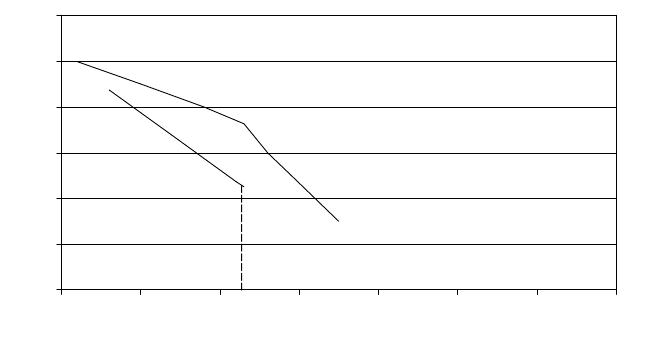
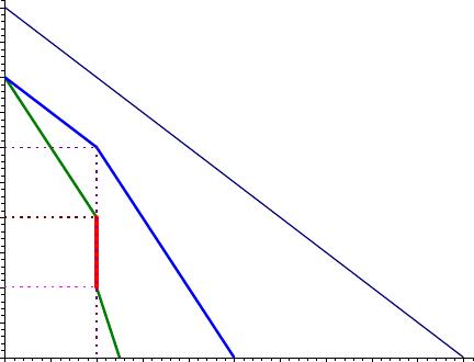
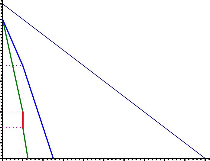
11. a. This firm controls 40% of the market (this is easily seen given P = $0).
b. The current price is $6, the intersection of followership and non-followership demand.
c. Panel B depicts a market in which niche players have a stronger brand identity.
In Panel A we see that the firm would control the entire market at any price below $2.
In Pane B we see that even at a price of $0, the firm only controls 80% of the market.
One can infer that at least some customers of the alternative varieties are willing to resist
switching even at a very low price in Panel B, but not in Panel A.
12. a. Inverse demand for firm A is: P = 10 – 2Q.
b. Demand at a price of $6 is obtained by setting P = 6 in the above and solving for Q:
6 = 10 – 2Q. This means that Qb = 2.
c. For prices above $6 market share will decline and for prices below $6 market share will remain
constant (at 50%).
d. This must be done in two parts:
Above P = $6 (and for Q < 2): P = 8 – Q.
Below P = $6 (and for Q > 2): P = 10 – 2Q.
Note: At P = $6, both demand curves have Q = 2.
13. a. MR has the same intercept and twice the slope as inverse demand so:
MR(Q) = 8 – 2Q for Q ≤ 2.
b. MR(Q) = 10 – 4Q for Q ≥ 2.
c. MR = MC= 3 occurs at Q > 2 using the MR equation in part E.
But this equation is only true for Q ≤ 2.
d. Similarly, MR = MC = 3 occurs at Q < 2 using the MR equation in part F.
But this equation is only true for Q ≥ 2.
MC = 3 passes through the jump discontinuity in MR.
In this instance, it makes sense for the firm to produce 2 units of output.
If instead MC = $4, then MR = MC occurs at Q = 2 given the MR curve associated with part E.
The firm should maintain a production of 2 units of output.
If instead MC = $2, then MR = MC occurs at Q = 2 given the MR curve associated with part F.
The firm should maintain a production of 2 units of output.
This is an example of “sticky prices”
The idea is that costs can vary and an oligopolistic firm may wish to maintain price (and
quantity) in order to not upset the oligopolistic bargain.
Copyright © 2014 Pearson Education, Inc.
Pricing and Output Decisions: Monopolistic Competition and Oligopoly101
$0
$1
$2
$3
$4
$5
$6
$7
$8
$9
$10
012345678910
The jump discontinuity in MR is shown in red in the diagram. If marginal cost passes anywhere
through this gap the appropriate output is Q = 2.
This implies that prices are “sticky” because they do not change despite a range of changes in
marginal cost.
14. The hallmark of kinked demand is that marginal revenue has a jump discontinuity at the kink
output level.
Given the assumption delineated above that the price intercept is lower for the portion of the
demand curve above $6 if the market share is higher, this means the kink is less pronounced for
smaller market share firms.
A smaller kink means a smaller jump discontinuity in the marginal revenue curve.
In this instance the jump is $1 rather than $2 (as it was in Question 19).
Answers for specific parts are as follows based on a 25% market share.
(12 take 2)
a. Inverse demand for firm A is: P = 10 – 4Q.
b. Demand at a price of $6 is obtained by setting P = 6 in the above and solving for Q:
6 = 10 – 4Q. This means that Qb = 1.
c. For prices above $6 market share will decline and for prices below $6 market share will remain
constant (at 25%).
d. This must be done in two parts:
Above P = $6 (and for Q < 1): P = 9 – 3Q.
Below P = $6 (and for Q > 1): P = 10 – 4Q.
Note: At P = $6, both demand curves have Q = 1.
(13 take 2)
a. MR has the same intercept and twice the slope as inverse demand so:
MR(Q) = 9 – 6Q for Q ≤ 1.
b. MR(Q) = 10 – 8Q for Q ≥ 1.
c. MR = MC= 3 occurs at Q = 1 using the MR equation in part E.
Therefore produce at Q = 1 since MR = MC.
If instead MC = $4, then MR = MC occurs at Q = 0.5 given the MR curve associated with part
E. The firm should reduce production to 1/2 unit of output.
Copyright © 2014 Pearson Education, Inc.
Pricing and Output Decisions: Monopolistic Competition and Oligopoly102
If instead MC = $2, then MR = MC occurs at Q = 1 given the MR curve associated with part F.
The firm should maintain a production of 1 units of output.
The price is less sticky for the 25% market share than the 50% market share firm.
This provides a rationale for one of the commonly observed outcomes in oligopolistic markets:
– Small market share firms often have more price flexibility than large market share firms.
10
1
1
0.25
6
Q
0
4
4
10
Suppose we believe that a larger market share firm will lose market
more quickly than a small market share firm — they are niche players
25
0
1
1
$0
$1
$2
$3
$4
$5
$6
$7
$8
$9
$10
0 1 2 3 4 5 6 7 8 9 10
Instructor note: The Excel App has sliders that allow you to vary market share as well as a
variety of other factors.
This graph is worth showing using overhead projection as it provides a strong visual image that
ties these problems together.
15. a. Monopolistic competition: different prices mean that we have a differentiated product market.
LR equilibrium means no incentive to change and free entry and exit.
b. P=AC in equilibrium; AVC=AC-AFC, AFC=FC/Q=500/100=5 for all firms. Therefore:
Salamandra’s Genoa’s Domino’s Four Star
AVCs=$6.00, AVCg=$6.00, AVCd=$4.00, AVC4=$3.00
c. No, they are not; with LR equal in monopolistic competition, each firm earns zero profits.
d. (P-MC)/P=1/elasticity. Given P and elasticity given we solve for MC in each case:
Salamandra’s Genoa’s Domino’s Four Star
MCs=$6.00, MCg=$7.00, MCd=$4.00, MC4=$3.00
e. If MC<AVC then AVC is decreasing, if MC>AVC then AVC is increasing. Comparing MC and
AVC for each firm we find:
Salamandra: flat; Genoa’s: up; Domino’s: flat; Four Star: down
Copyright © 2014 Pearson Education, Inc.
Pricing and Output Decisions: Monopolistic Competition and Oligopoly103
f. All four are on the downward part of their AC. In equilibrium, AC is tangent to downward
sloping demand in LRMCE.
g. The Lerner index (also known as the inverse elasticity rule), used in part d above, answers this
question. Based on elasticity, we know that Genova’s has the smallest markup (4/11th=36.4%);
Domino’s has the largest markup (55.6%).
Copyright © 2014 Pearson Education, Inc.