
CHAPTER 6 AND APPENDICES
THE THEORY AND ESTIMATION OF PRODUCTION
QUESTIONS
1. The short run production function contains at least one fixed input. In the long run production
2. The law of diminishing returns: As additional units of variable input are added to a fixed input, at
This law is considered a short-run phenomenon in economic theory because it requires at least one
of the inputs used by the firm to be held constant.
3. Stage I ends and Stage II begins at the point of maximum AP. Stage II ends and Stage III begins at
4. Adhering to the MRP=MLC (or MRP=MFC) rule is an example of equalizing at the margin. As
Once MLC exceeds MRP, it no longer pays for the firm to do so if it wants to maximize its
5. Returns to scale is a measure of the increase in a firm’s output relative to a proportionate increase in
6. Perhaps the firm is not following the rule at first. However, after completing the program, the
7. If marginal product is greater than average product, average product increases. If it is less than
average product, average product decreases. If it is equal to average product, then average product
Copyright © 2014 Pearson Education, Inc.
The Theory and Estimation of Production 41
8. A firm may find itself in Stage I or III of its short run production function simply because of the
9. It is sometimes difficult to measure productivity, particularly for individuals. Economists use fairly
broad measures of productivity such as the market value of output divided by the number of
a. Education: An obvious quantitative measure of teacher productivity would be number of
b. Government: Number of forms processed, number of inquiries answered, number of audits
c. Manufacturing: Manufacturing industries conform very closely to the traditional economic
d. Finance and Insurance: It is little easier to measure output here than in the case of education
and government. The only caution is that output in terms of customers served may not be as
10. A question that we found opens the class up to some interesting discussion. We leave the answer for
11. The two regression methods used in estimating production functions are the cross-section and
In a time-series analysis, the analyst must assure himself/herself that there have been no
technological changes in the plant during the time-frame of the study. If any of the data used in this
Copyright © 2014 Pearson Education, Inc.
The Theory and Estimation of Production 42
12. Since we will be studying a single steel mill, we will employ a time-series regression analysis. We
will collect monthly data over a period of three years when there was little or no change in the
The call center and the steel mill would ostensibly involve the same general categories of inputs:
labor and capital. For example, in the case of the call center, the capital would be the office
facilities, the telephone premise equipment and computers and all of the other computers and
Key learning point for students: the challenge of measuring the output of a production function for
a service rather than for a good.
13. A Cobb-Douglas function of the form Q = aLbK1-b exhibits constant returns to scale. If the function
14. If b is less than 1, the production function exhibits diminishing marginal returns.
Copyright © 2014 Pearson Education, Inc.

The Theory and Estimation of Production 43
15. True. In a Cobb-Douglas function with constant returns to scale, the sum of the coefficients is 1.
16. If Q = quantity produced and V is the quantity of the variable factor, then the equation Q = bV – cV2
In order to show a production function with both increasing and decreasing returns, a cubic function
is necessary:
Q = bV + cV2 – dV3.
Copyright © 2014 Pearson Education, Inc.
The Theory and Estimation of Production 44
PROBLEMS
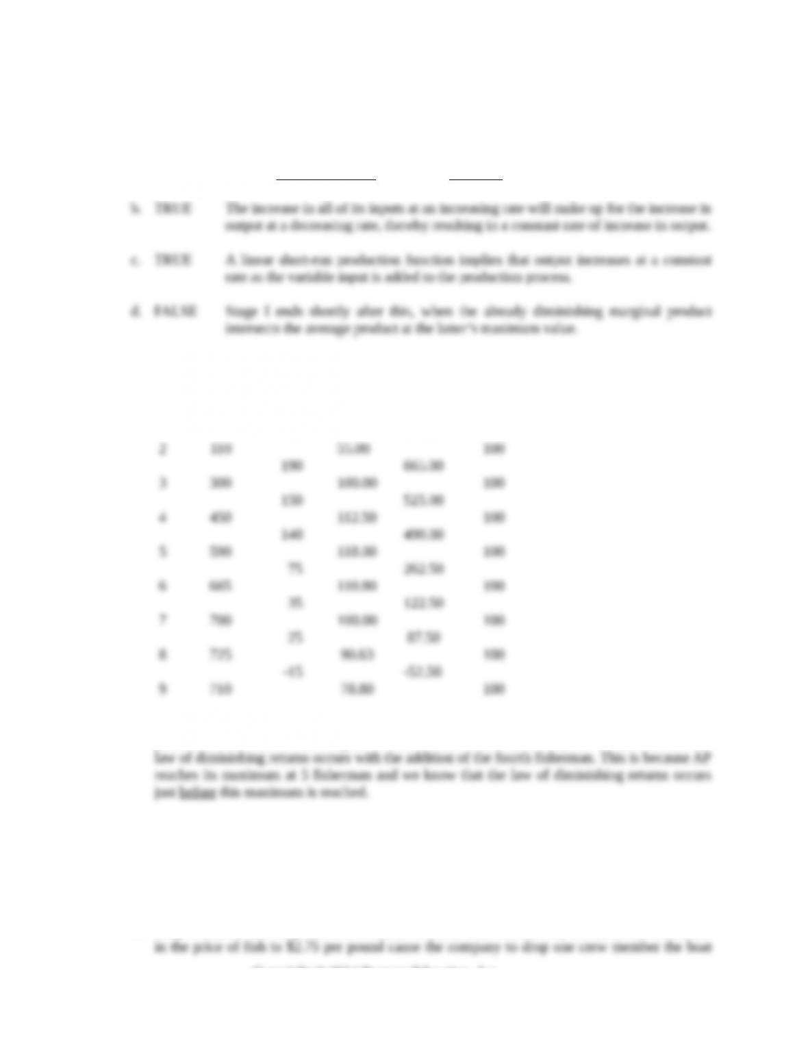
1. a. FALSE A firm’s marginal product will start to decrease.
2. L Q MP AP MRP W
0 0
50 175.00
1 50 50.00 100
60 210.00
a. Based on the knowledge of the law of diminishing returns in relation to the three stages of
production and without knowing the MP for the first three fishermen, we can surmise that the
b. Stage I: 1 to 5 units of L
Stage II: 5 to 8 units of L
Stage III: 8 units of L and above
c. 7 L
d. They would have to drop one crew member from the boat and use only 6 fishermen. A decrease
Copyright © 2014 Pearson Education, Inc.
The Theory and Estimation of Production 45
e. Because the maximum catch in the short run for the boat is 725 pounds, the company would
Instructors may ask students to think of other possibilities.
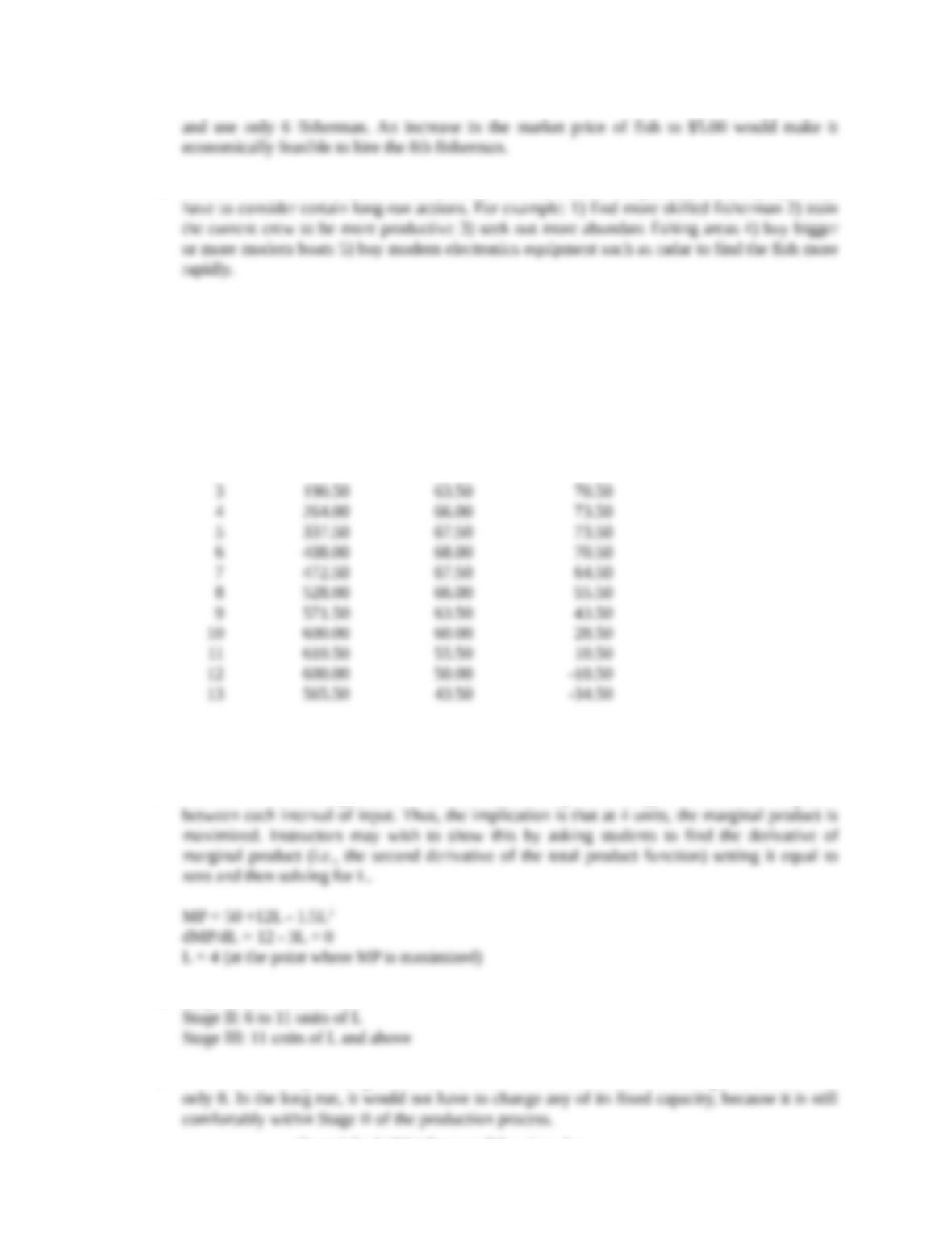
3. Based on the equation Q = 50L + 6L2 – .5L3, we can generate the following short run production
schedule:
Variable Factor Total Product Average Product Marginal Product
0 0.00
1 55.50 55.50 55.50
2 120.00 60.00 64.50
(Please note that the marginal product in this schedule was calculated as the change in total product,
as the variable factor is changed by one unit.)
a. The law of diminishing returns occurs at 4 units of input. Actually, the MP should be placed
b. Stage I: 1 to 6 units of L
c. 9 workers. If the price drops to $7.50 the firm will have to consider reducing its labor force to
Copyright © 2014 Pearson Education, Inc.
The Theory and Estimation of Production 46
Copyright © 2014 Pearson Education, Inc.
The Theory and Estimation of Production 47
4. Vehicles Mechanics Total Cost*
100 2.5 $625,000
*There are obviously other costs involved in this operation. In this example, we are assuming that
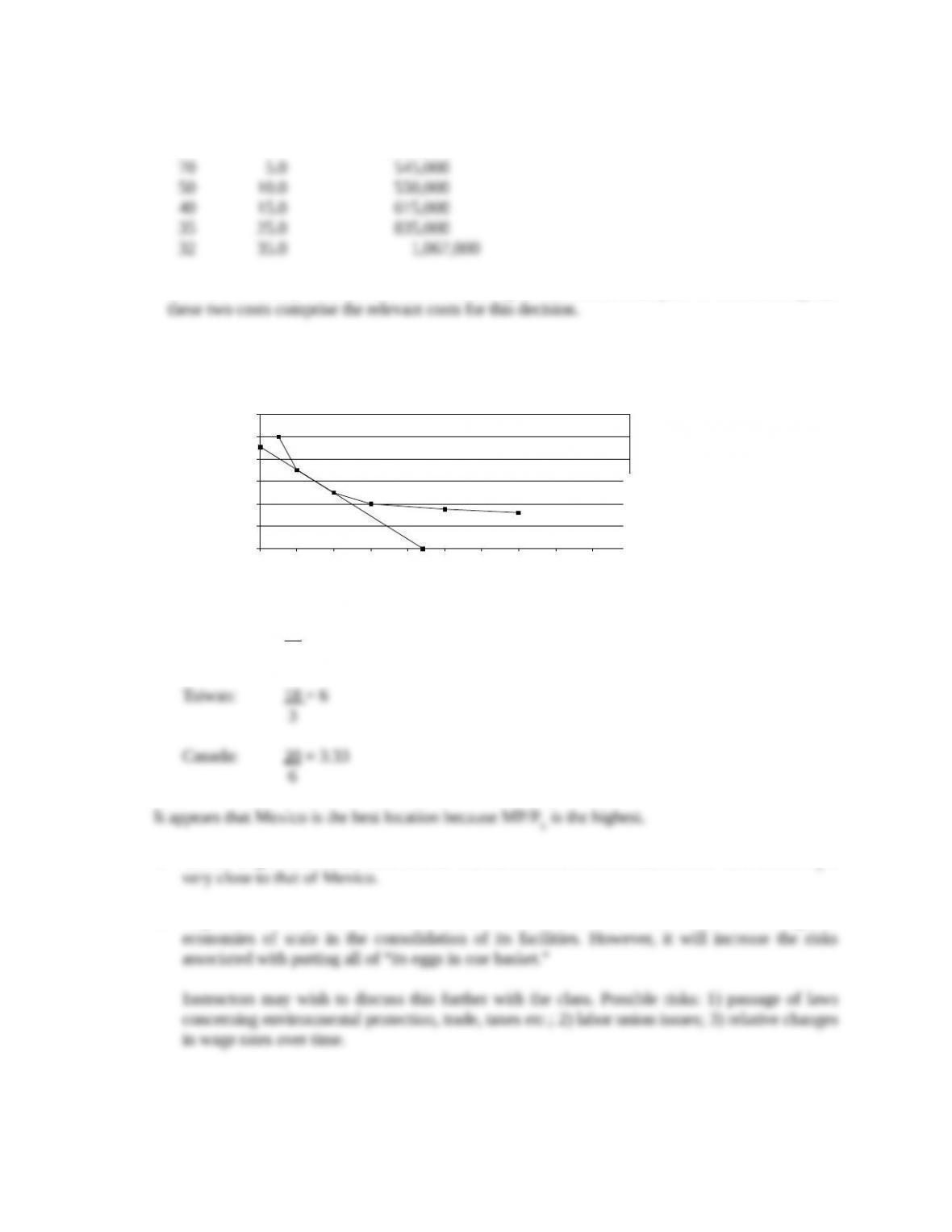
a. The use of 70 vehicles and 5 mechanics will minimize total cost.
b.
Figure 6.1
5. a. Mexico: 10 = 6.67
1.5
b. Taiwan might be a better location than Mexico because its overhead is lower and its MP/PL is
c. Regardless of which location is chosen, the manufacturer should receive some advantages of
Copyright © 2014 Pearson Education, Inc.
Optimal point
Second best point *
Q
0
20
40
60
80
100
120
0 5 10 15 20 25 30 35 40 45 50
Mechanics
Vehicles
*This point represents a total cost
of $550,000, but is difficult to
differentiate on the graph from the
optimal point representing
$545,000.
The Theory and Estimation of Production 48
6. a.
MRP
L Q MP AP (P=$5)
0
1 5.5 5.5 5.5 27.50
2 10.0 4.5 5.0 22.50
Figure 6.2
b. 5 workers
c. No, because the 6th person has an MRP of $2.50. In order to hire this person, the wage rate
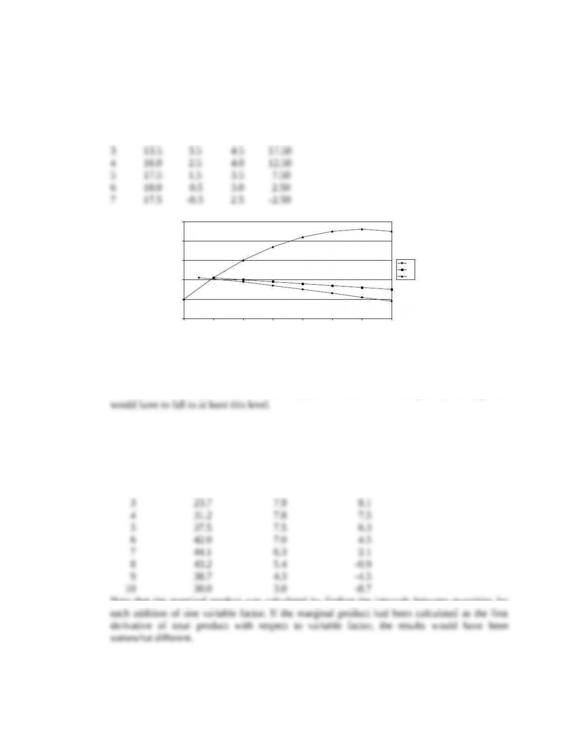
7. a. and b.
Variable Factor Total Product Average Product Marginal Product
0 0.0
1 7.5 7.5 7.5
2 15.6 7.8 8.1
Note that the marginal product was calculated by finding the intervals between quantities for
Copyright © 2014 Pearson Education, Inc.
–5
0
5
10
15
20
0 1 2 3 4 5 6 7
L
MP
AP
Q
The Theory and Estimation of Production 49
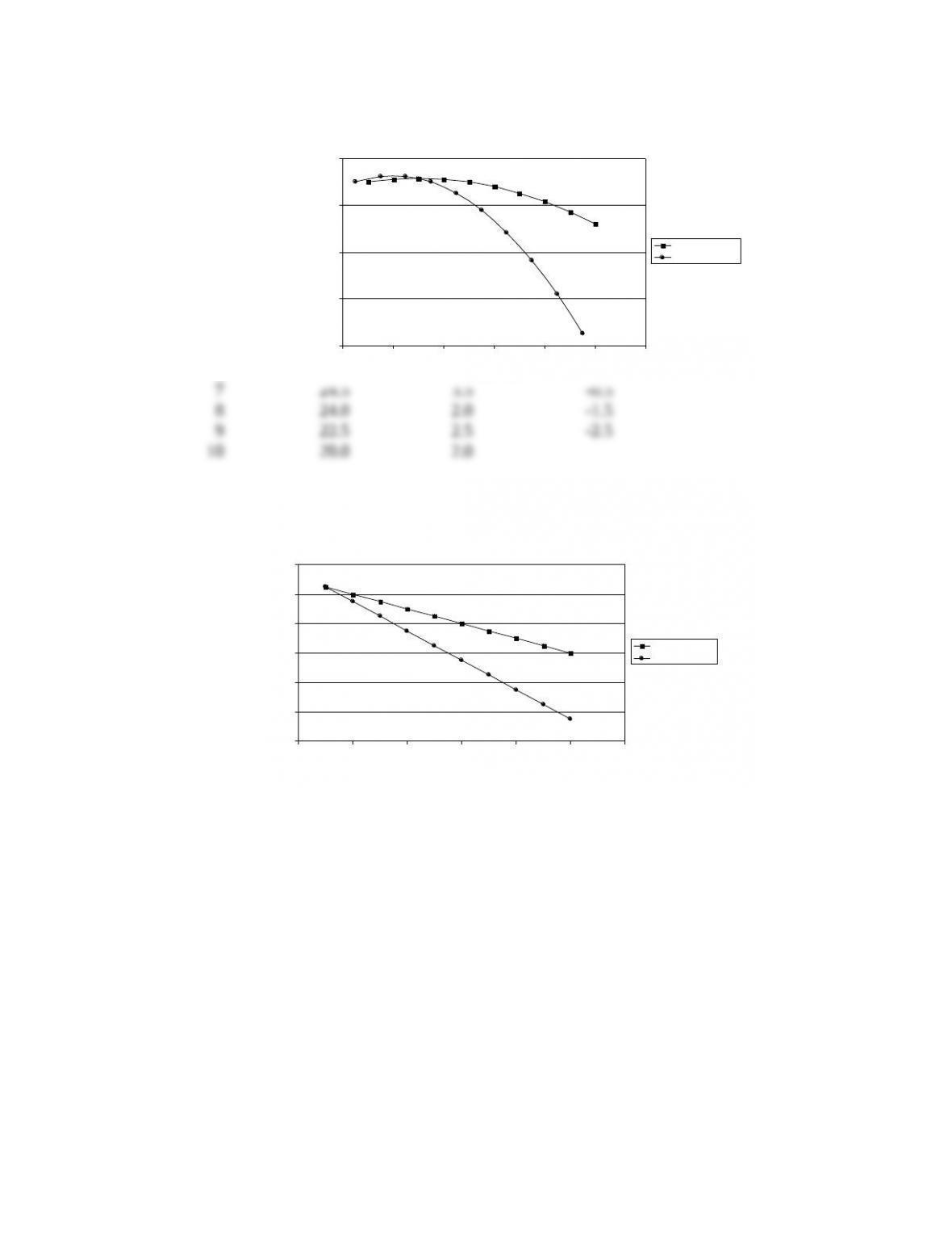
c.
Figure 6.3
8. a. and b.
Variable Factor Total Product Average Product Marginal Product
0 0.0 6.5
1 6.5 6.5 5.5
2 12.0 6.0 4.5
3 16.5 5.5 3.5
4 20.0 5.0 2.5
5 22.5 4.5 1.5
6 24.0 4.0 0.5
The marginal product was calculated by the same method as in problem 2.
c.
Figure 6.4
Copyright © 2014 Pearson Education, Inc.
–10
–5
0
5
10
0 2 4 6 8 10 12
Va riable Factor
Average Product
Ma rginal Product
AP, MP
–4
–2
0
2
4
6
8
0 2 4 6 8 10 12
Variable Factor
Average Product
Marginal Product
AP, MP
The Theory and Estimation of Production 50
d. The function in problem 7 was a cubic function, while in this problem it is a quadratic function.
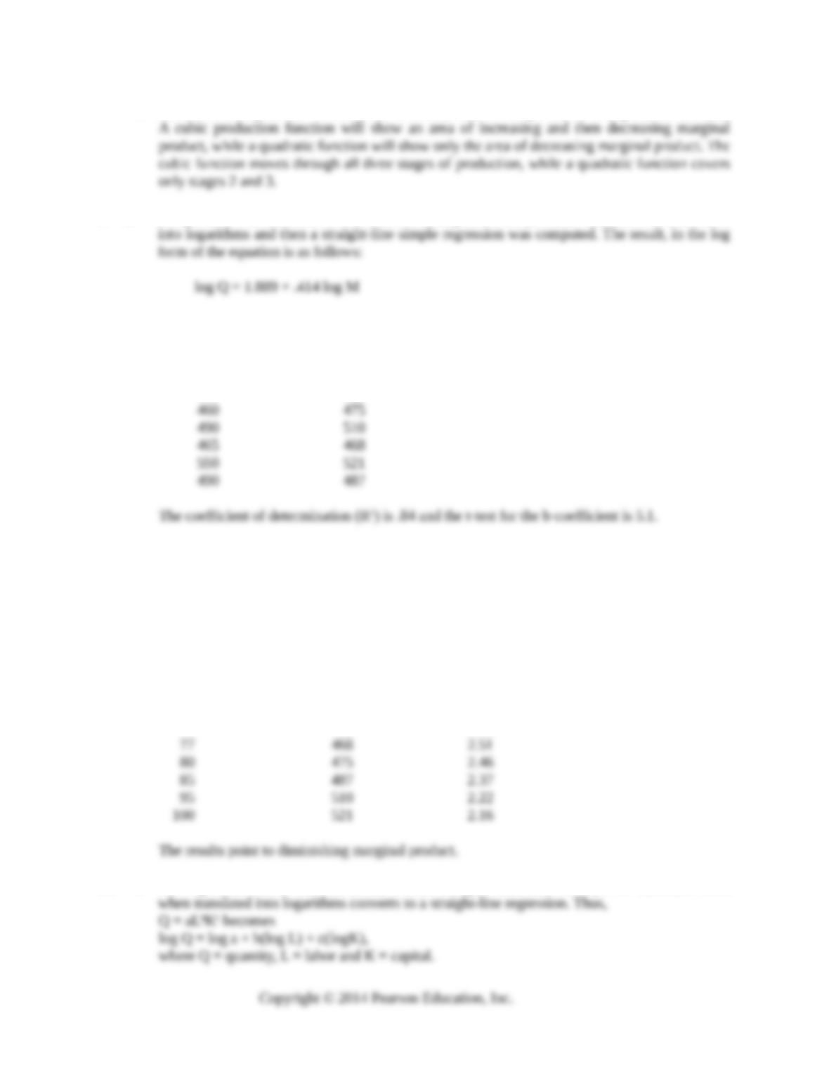
9. a. A regression was calculated for the observations given in the problem. The data were translated
The estimated quantities compared to the actuals (when anti-logs are taken) are:
Actual Quantity Estimated Quantity
450 450
430 422
b. The above results are fairly satisfactory. The coefficient of determination is relatively high, and
the t-statistic for the slope coefficient is significant. The estimated results, shown above, are, in
most instances, quite close to the actuals. Probably, some improvement could be obtained if a
second variable input, such as utility bills, had been utilized as a second independent variable.
c. The formula for marginal product is bQ/M. The marginal products (based on estimated
quantities) are shown below:
Materials Estimated Quantity Marginal Product
60 422 2.91
70 450 2.66
10. a. The regression which was calculated, a Cobb-Douglas function, was a power function, which
The Theory and Estimation of Production 51
b.
Labor Capital Actual Quantity Estimated Quantity
250 30 245 226.1
270 34 240 251.6
c. The sum of the two coefficients, b and c, is greater than 1 (.825 + .346 = 1.171). Therefore, the
d. The elasticities of production of the two factors are their respective coefficients, b and c.
e. The marginal product of labor is decreasing since the coefficient b is less than 1.
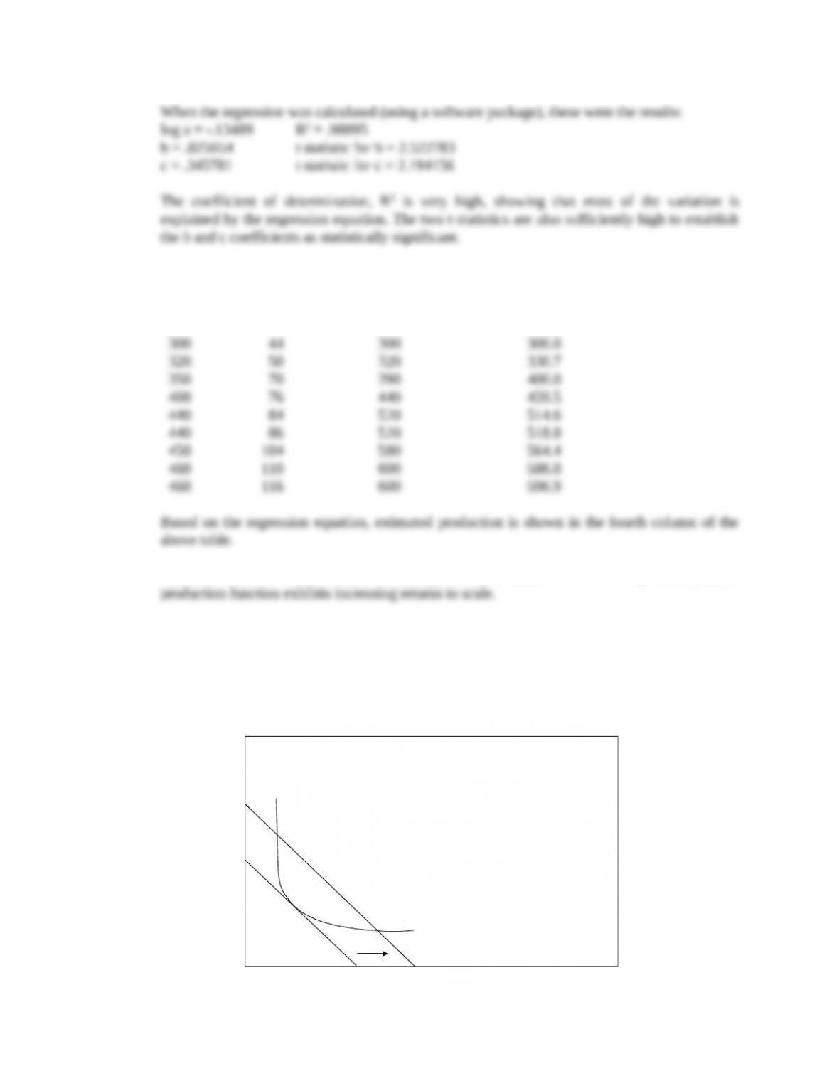
11. a.
Copyright © 2014 Pearson Education, Inc.
Y
X
The Theory and Estimation of Production 52
Figure 6.5
b.
Figure 6.6
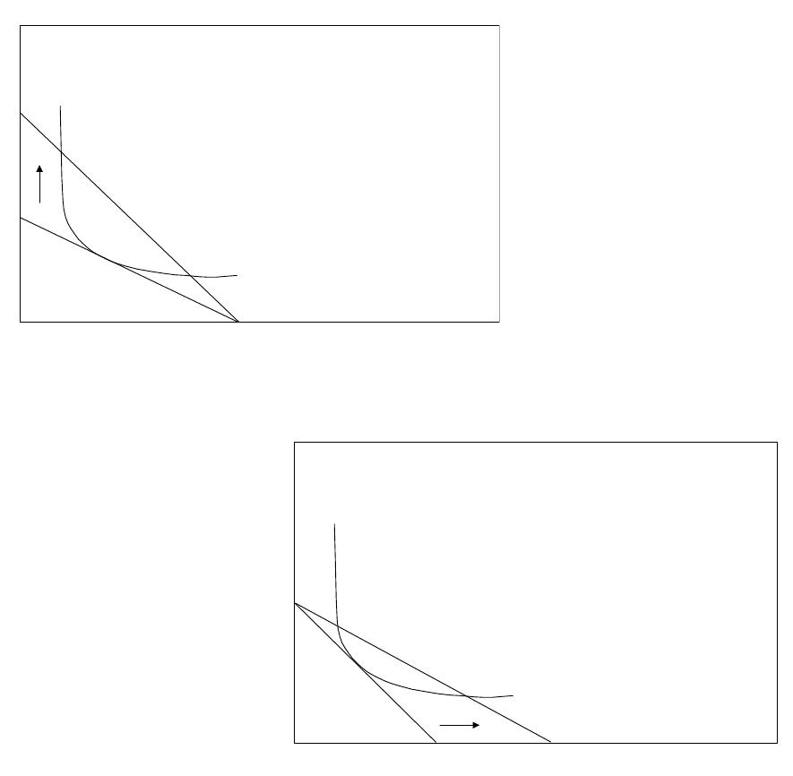
c.
Figure 6.7
Copyright © 2014 Pearson Education, Inc.
Y
X
Y
X
The Theory and Estimation of Production 53
d.
Figure 6.8
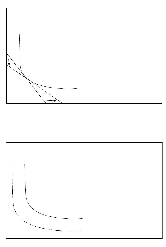
e.
Figure 6.9
Copyright © 2014 Pearson Education, Inc.
Y
X
Y
X
Q
1
Q
2
The Theory and Estimation of Production 54
f.
Figure 6.10
12. a. The numbers are the same as those in text Table 7B.1. This question gives an opportunity for
students to see for themselves how this function can generate such numbers.
13. a. CRTS
14. a. This is an IRTS production function.
b. Because this function is expressed in the table in a discrete rather than continuous manner, there
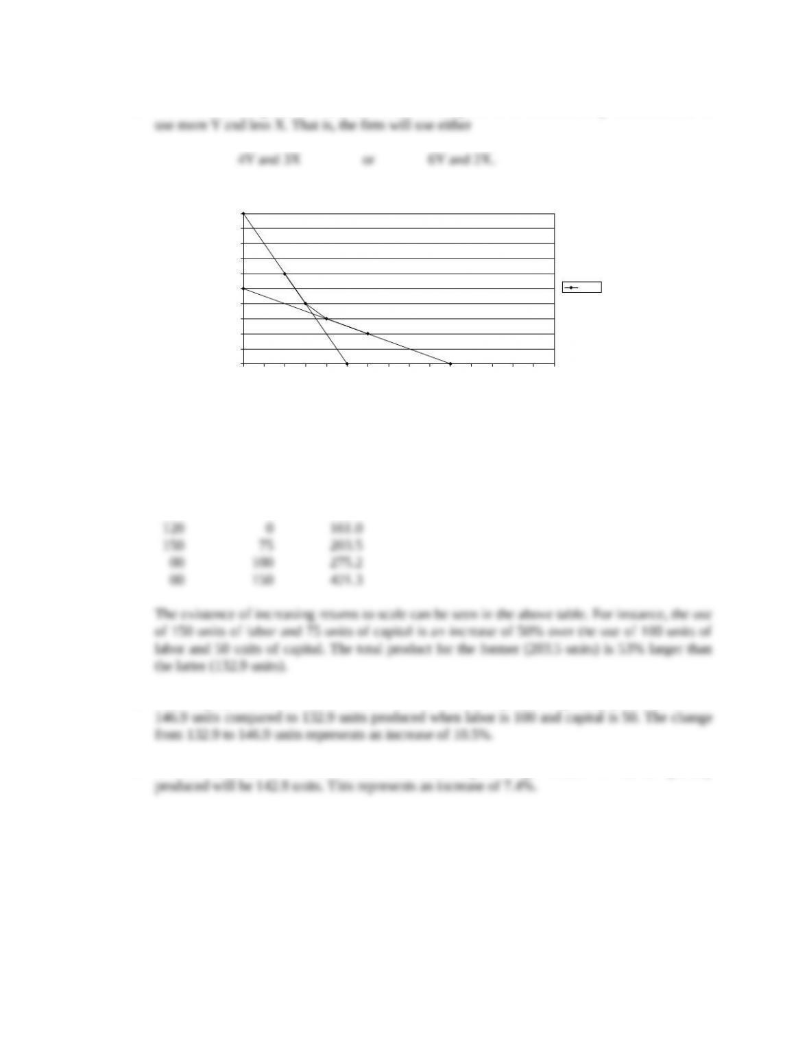
2Y and 6X or 3Y and 4X.
Copyright © 2014 Pearson Education, Inc.
Y
X
Q
1
Q’
1
The Theory and Estimation of Production 55
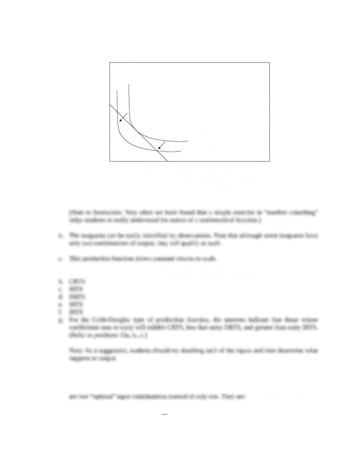
c. A decrease in the price of Y and an increase in the price of X will obviously cause the firm to
d.
Figure 6.11
15. a. Since the coefficients add to more than one (.75+.3 = 1.05), this production function exhibits
increasing returns to scale.
b. Labor Capital Quantity
100 0 132.9
c. With employment of 110 units of labor and 55 units of capital, the quantity produced will be
d. If labor increases to 110 units from 100, while capital usage remains at 50, the quantity
Copyright © 2014 Pearson Education, Inc.
0
1
2
3
4
5
6
7
8
9
10
0 1 2 3 4 5 6 7 8 9 10 11 12 13 14 15
X
Y
Q = 54
The Theory and Estimation of Production 56
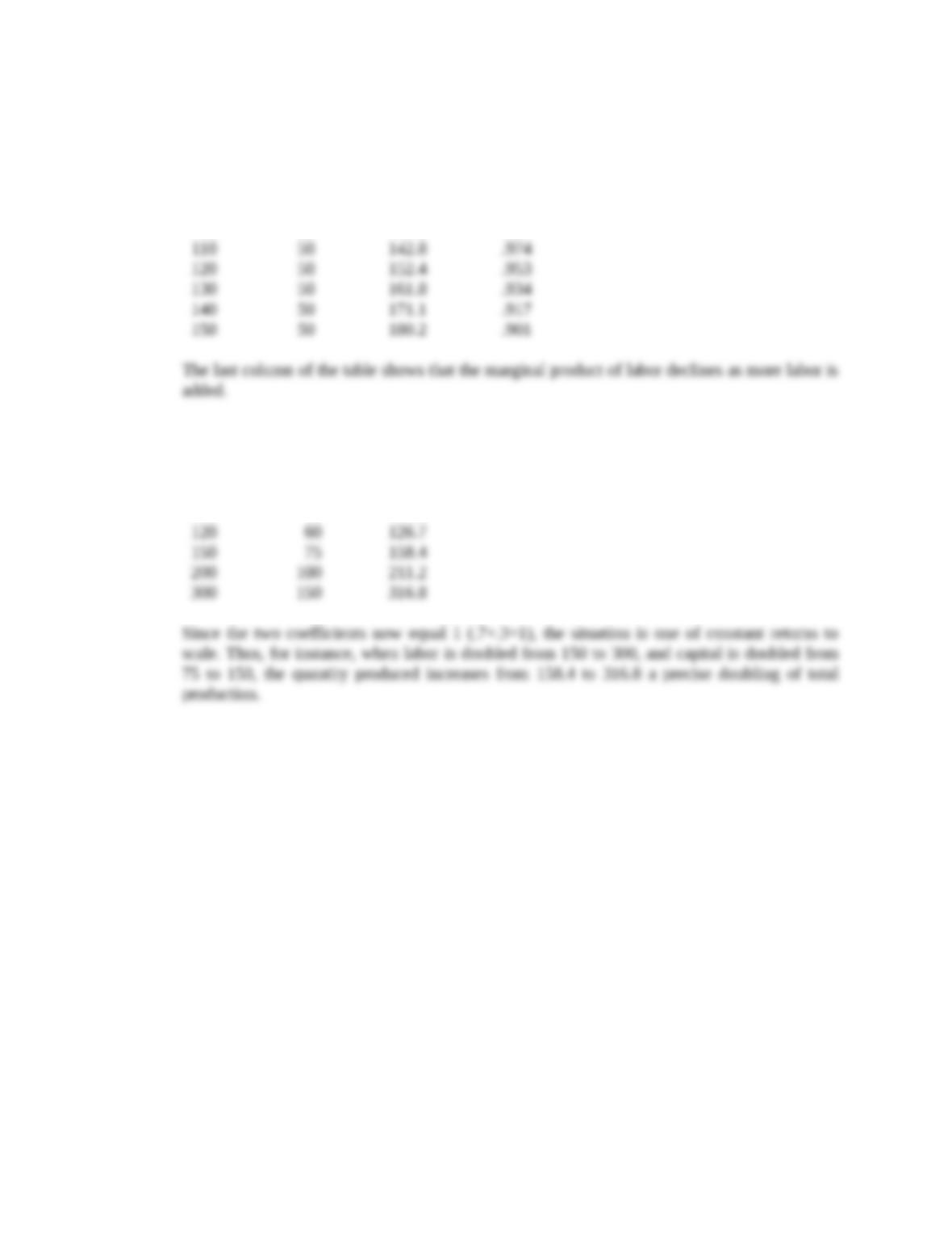
The table below shows the total product when labor is increased by intervals of 10 but capital
remains the same. The marginal product of labor is calculated at each point using the formula
bQ/L.
Labor Capital Quantity MP of Labor
100 50 132.9 .997
e. If capital were to increase by 10% from 50 to 55 while labor remains at 100, the quantity
produced would increase to 136.8, an increase of about 2.9%.
f. Labor Capital Quantity
100 50 105.6
Copyright © 2014 Pearson Education, Inc.