CHAPTER 5
DEMAND ESTIMATION AND FORECASTING
QUESTIONS
Demand Estimation
1. Time series data: Information concerning a particular variable over time at specified intervals (e.g.,
2. In both cases, as many of the price and non-price factors that influence demand should be included.
3. R2 is a measure of the explanatory power of the regression model. It is also referred to as a measure
of “the goodness of fit” (of the regression line through the scatter of data points). Specifically, it
Other factors held constant, time series data generally produce a higher R2 than cross-sectional data
because both dependent and independent variables often move together over time simply because of
4. a. State the null hypothesis and the alternative hypothesis.
5. The F-test is a measure of the statistical significance of the entire regression equation. If it is used in
simple regression (i.e., for a regression equation with only one independent variable), then in effect
6. Multicollinearity occurs when two or more independent variables in a regression equation are
highly correlated with each other. An indication of this problem occurs when a regression equation
7. The identification problem refers to the difficulty of clearly identifying the demand equation
Forecasting
1. Not necessarily. While more accuracy is better than less, a cost is usually involved in making
2. Qualitative: usually not based on quantitative historical data although results may be
3. a. Jury of executive opinion. Opinions come from experts in the forecast area, but in a panel
b. Delphi method. Forecasts are made by experts. The experts’ opinions are usually obtained over
the telephone or by writing, and are carried out by a sequential series of questions and answers.
c. Opinion polls. These are surveys conducted with population samples that are not experts but
whose activities may determine future events. Since only samples are surveyed, it is essential
4. a. Manufacturers’ new orders and nondefense capital goods are spending plans and will
b. The index of industrial production reflects the actual economic activity at the time it is reported.
5. A major problem is that, while leading indicators are a fairly good forecaster of changes in
economic activity, they are not reliable at forecasting the timing of troughs or peaks. The lead time
6. From the beginning of 1626 to the end of 2007 is 383 years, or 766 semiannual periods. At 3%
7. The compound growth rate method will give reasonable results if the growth rate of the past is
8. Moving average projections: A moving average of past data is used to forecast the next period. The
number of past observations to include in the moving average must be specified. Thus, if a 1996
9. Naive forecasting models forecast the future trends without explaining the reason for these changes.
10. The following data would probably be important:
11. The data appear to show that a recovery got under way in the last months of 2001 and into 2002.
PROBLEMS
Demand Estimation
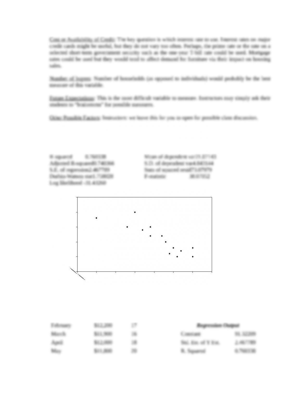
1. Price: Average price of the furniture. If the demand for different models or types (e.g., dining room,
bedroom, living room furniture) is estimated, then the average price of each type must be used.
10
15
20
25
30
35
9500 10000 10500 11000 11500 12000 12500 13000
P
Q
0
0
2. Variable Coefficient Std. Error T–Stat. 2-Tail Sig.
C 91.322086 11.404689 8.0074157 0.000
Price-0.0060524 0.0009809 -6.1701311 0.000
Month Price Quantity
January $12,500 15
June $12,500 18 No. of Observations 14
July $11,700 22 Degrees of Freedom 12
950
0
1000
0
1050
0
1100
0
1150
0
1200
0
1250
0
1300
0
1
0
1
5
2
0
2
5
3
0
3
5
Q
P
0
0
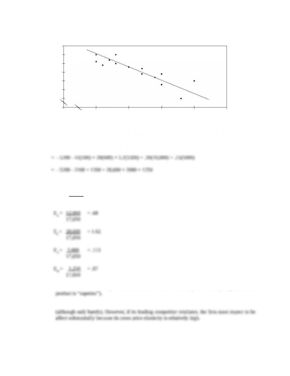
Scatter Graph—Automobile Dealership
3. Q= – 5200 – 42P + 20PX + 5.2I + .20A + .25M
Q= 17,650
a. EP = – 21,000 = -1.18
17,650
b. This firm should be very concerned because income elasticity is relatively high (i.e., the
c. This firm might want to cut its price to increase its sales because the product is price elastic
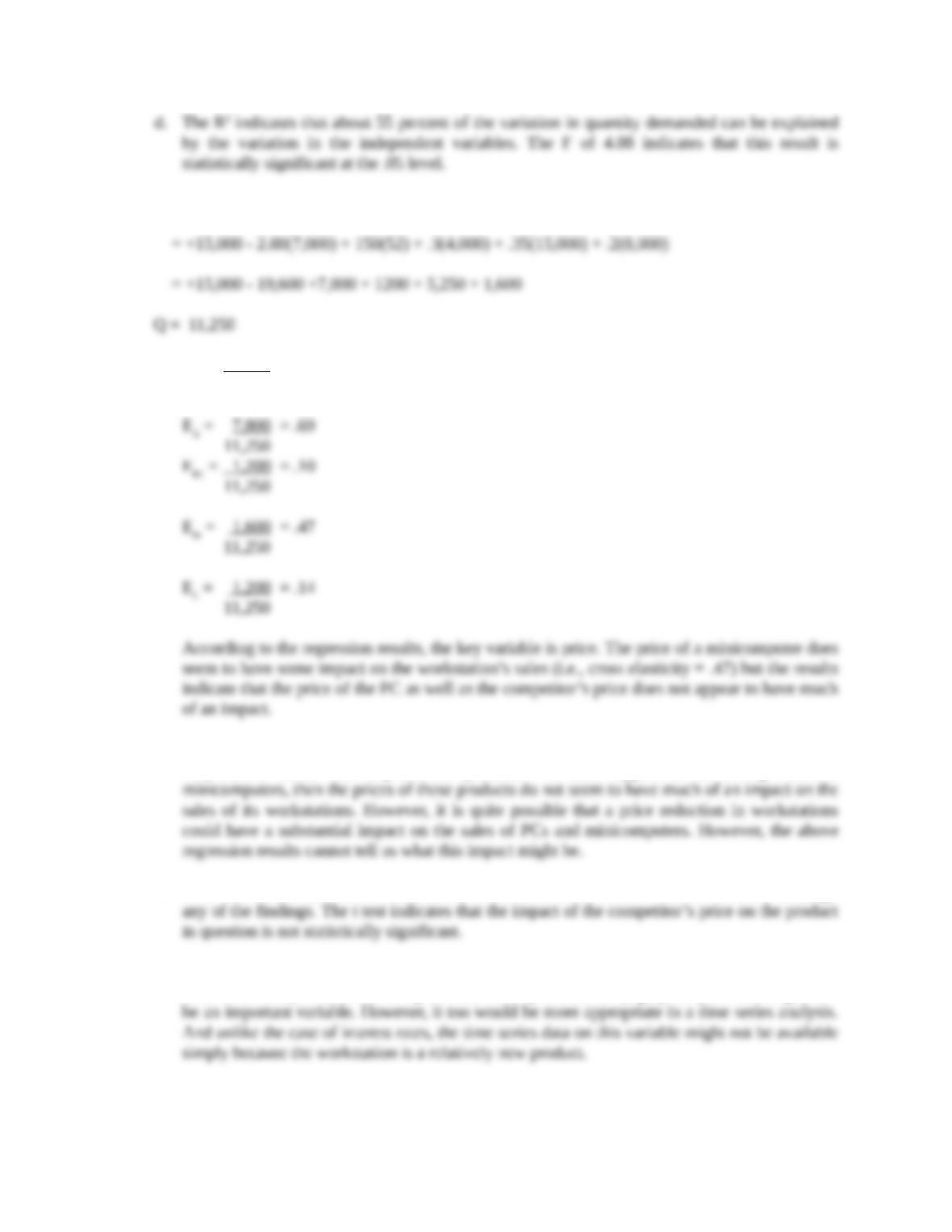
4. Q = +15,000 – 2.80P + 150A + .3PPC + .35PM + .2PC
a. EP = 19,600 = -1.74
11,250
The results indicate that customers are extremely price sensitive. Therefore, the firm should be
very careful about how it prices the product. If it also happens to be selling PCs and
b. A one-tail test can be used for each of the variables. The use of a two-tail test would not change
c. Interest rates might well have an impact on sales. However, it would be more appropriate in a
time-series analysis of sales. The price relative to performance (e.g., price per MIP) might also
5. a. The coefficient of Pj (1.2) is greater than that of Pa (.75). This implies that consumers perceive
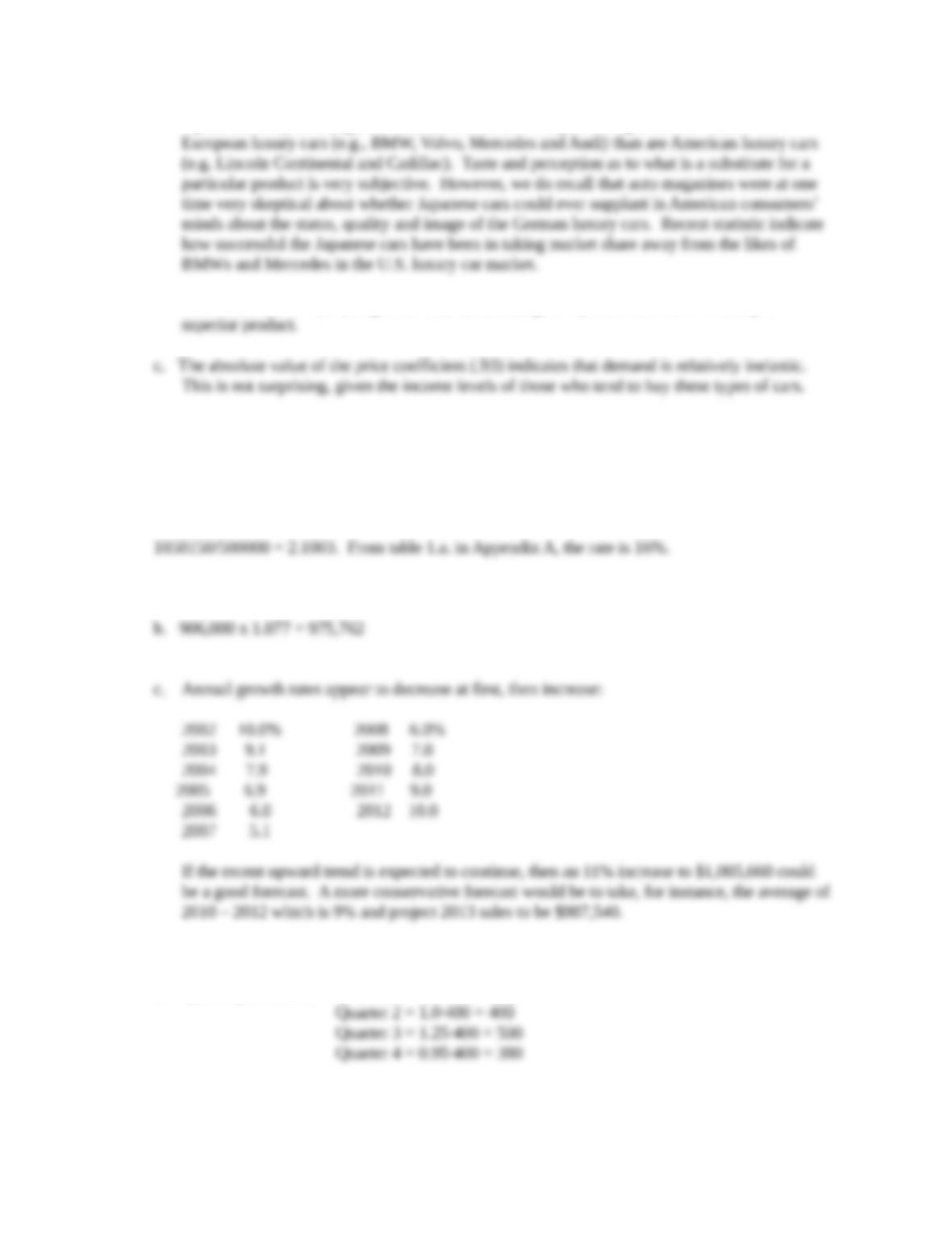
Japanese luxury cars (e.g., the Acura, Lexus and Infinity) as being close substitutes for
b. The coefficient of I (1.6) is greater than 1, indicating as expected that this is a luxury or
Forecasting
1. The compound growth rate is 16%. The answer can be obtained as follows:
2. a. 7.7%
3. a. In 2013, t = 6 so Q = 1,000 + 100•6 = 1,600
b. Quarterly sales are: Quarter 1 = 0.8·400 = 320
4.a. 16% (a more exact answer is 15.98%)
b. If growth calculated at 16%: 2013 1,012,680
c. 14% (more exact answer is 14.02)
d. If growth calculated at 14%: 2013 995,220
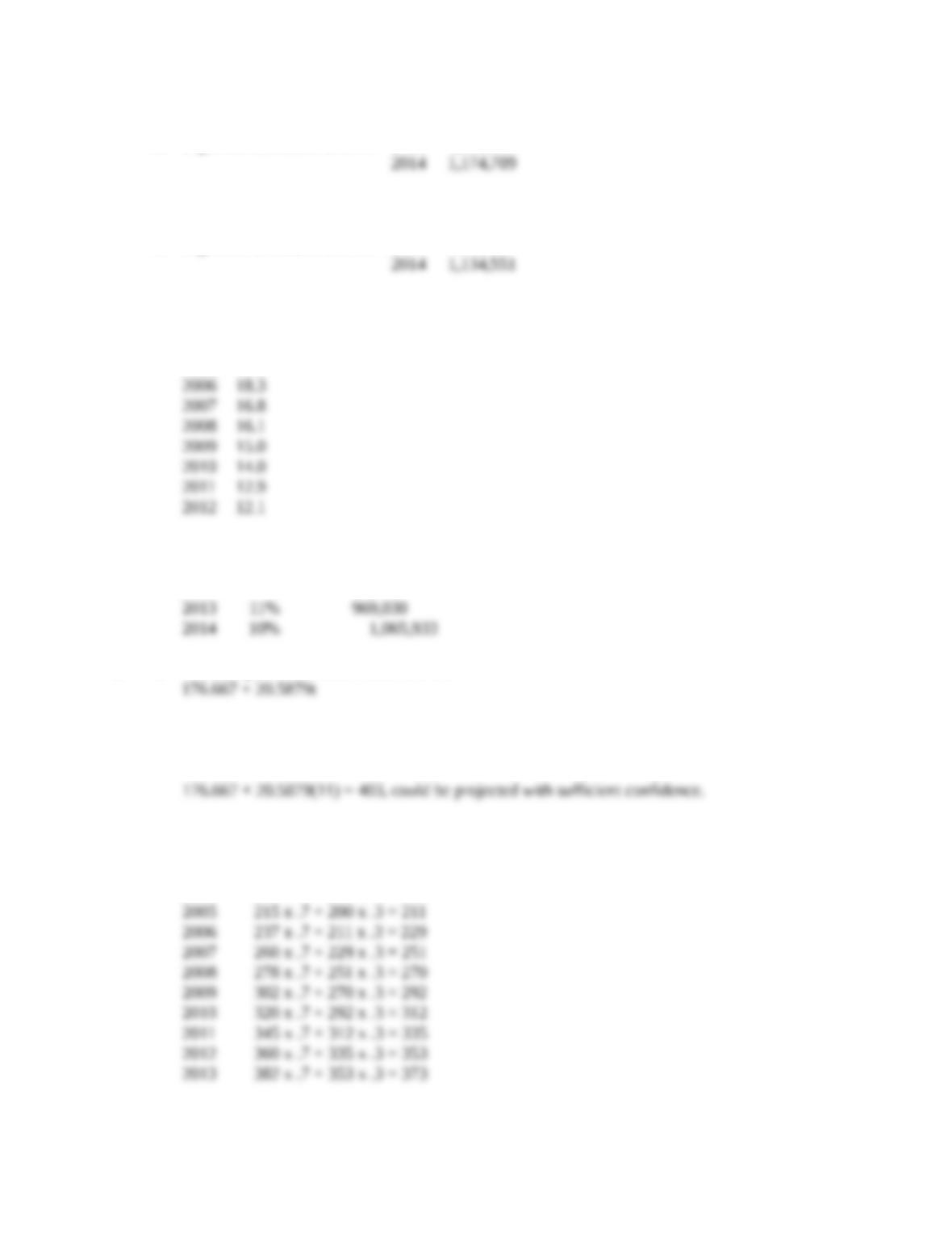
e. The annual growth rate in sales from 2004 to 2012 is decreasing:
2004 20.0%
2005 18.8
On average the decrease in the rate of growth was 1% point per year. If this trend were to
continue, the forecasts for 2013 and 2014 would be:
5. a. A least-square time-series trend line is:
The past 10 years describe a straight line. Thus, if it is expected that 2013 would continue on a
similar trend, then
b. Using exponential smoothing for the entire series, with a factor of 0.7, would give the
following result:
2004 200 x .7 + 200 x .3 = 200
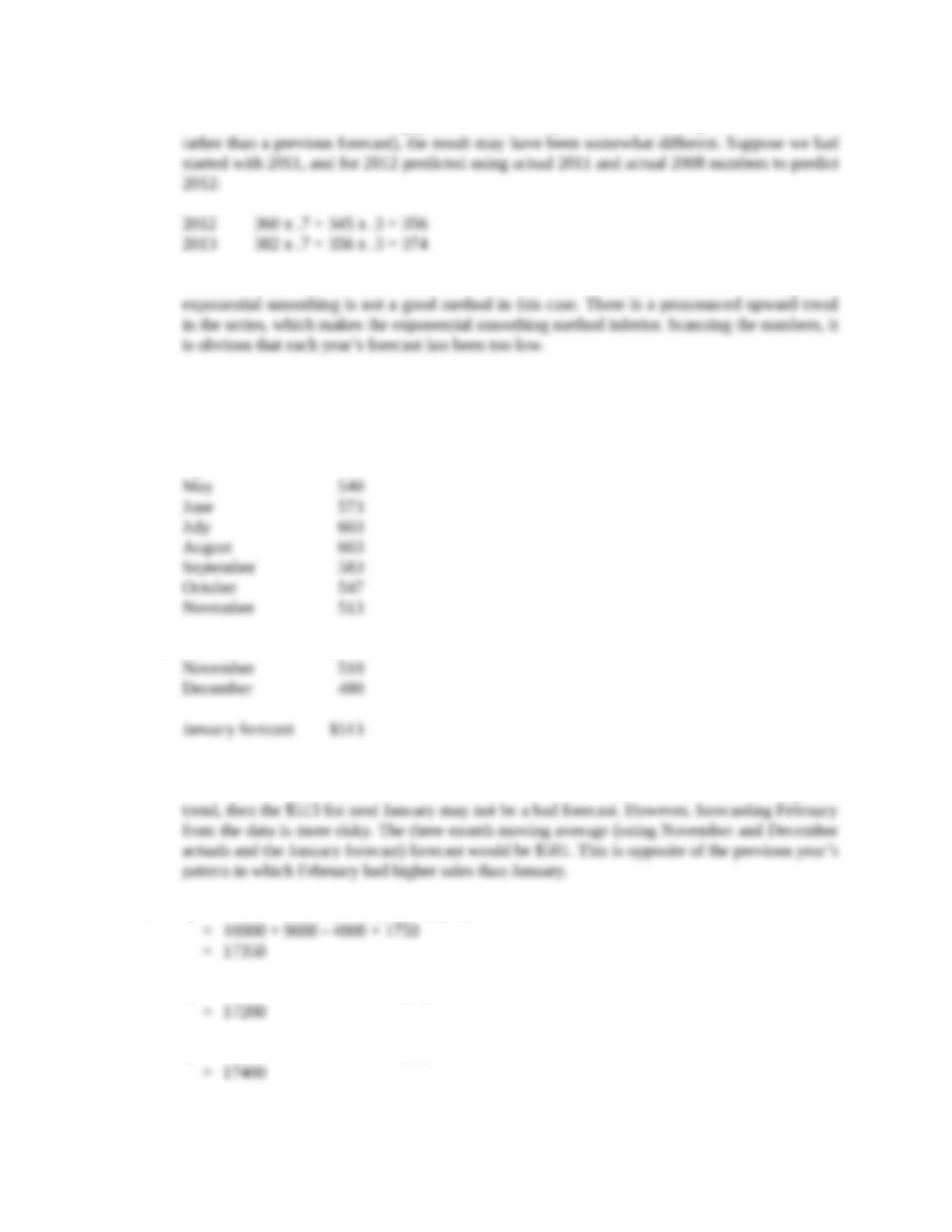
If we had started the smoothing procedure just one period back (utilizing the actual number
It can be seen that the difference in the two forecasts is quite small. Forecasting with
6. a. Three-month centered moving average:
February $513
March 517
April 520
b. October $550
c. In general, since the annual pattern is quite seasonal, the moving average forecast is not a good
one. It is difficult to say whether the January forecast is reliable. If there is an overall upward
7. a. Q = 10000 + 60(160) – 100(40) + 50(35)
b. Q = 10000 + 9600 – 4000 + 50(32)
Q = 10000 + 9600 – 4000 + 50(36)
c. Q = 10000 + 9600 – 100(37) + 50(32)
d. 60(160) = 9600
With an index of 140 rather than 160, quantity would decrease by 1200 units.
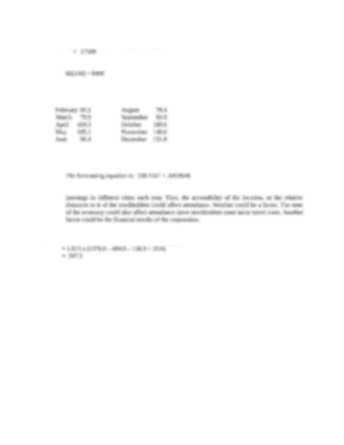
8. January 55.4 July 87.5
9. a. Expected attendance is 582.
b. Other factors should be taken into consideration. Many companies hold their stockholder
10. Q = 1.015 x [1376.0 – 17.1(40) – 3.7(37) + 4.2(8)]