CHAPTER 10
SPECIAL PRICING PRACTICES
QUESTIONS
1. False. This statement could be true if average cost were constant and completely variable with
2. An example of the equity argument is given by the medical profession, when certain (low income)
3. The higher is the demand elasticity the lower will generally be the mark-up. Thus, cigarettes and
4. Most probably, the price of coffee was the one which was raised, since presumably it has the lower
5. Both types of price leadership will occur in an oligopolistic industry. The case of barometric
6. Yes. In order to maximize the total profits of the cartel, the cartel will charge a monopoly price.
7. Conditions favorable to formation of cartel:
a. Small number of large firms.
Copyright © 2014 Pearson Education, Inc.
Special Pricing Practices 98
8. Yes. Monopolies can be created through regulation and licensing.
For instance, licensing is required of various professions, such as electricians, plumbers, doctors,
Natural monopoly conditions (large cost economies of scale over the entire range of output to meet
In the past, several industries were regulated, e.g., the airlines. Routes and fares were specified by a
government agency. Price competition did not exist.
It might also be said that other types of government regulations (however important they may be)
9. The Baumol model states that companies (in oligopolistic industries) have for their objective the
maximization of revenue subject to a minimum profit constraint.
The price charged by such companies would be lower than that of a profit maximizer and quantities
Revenue maximization may be important in some cases, particularly where a company tries to gain
10. Not in all instances, since these prices are charged at different times of the day where the costs of
11. If average variable costs are constant or nearly constant, then the methods will give same or similar
answers.
12. When two passengers sitting next to one another on an airplane have paid different prices for the
same trip, it would appear that this is an obvious example of price discrimination, and in some cases
Copyright © 2014 Pearson Education, Inc.
Special Pricing Practices 99
Further, there are significant swings in demand during different times in a week. Mondays,
Thursdays and Fridays appear to have more (business) traffic than the other days. Thus, lower price
13. No. Within a company, mark-ups can differ from product to product. Such price differences are
probably governed by differences in demand elasticity. Also, a company will change its prices and
14. a. Transfer pricing: a computer company which operates at different stages of production will
often employ transfer pricing. Suppose the product advances through four stages: manufacture
b. Psychological pricing: a price which would appeal to the public is established. For instance, a
product could be priced at $19.95 instead of $20, since the small difference creates an illusion
c. Price skimming: the producer of a new product (with no competition) will charge a higher
price. The price charged ideally would be along the demand curve (skims the demand curve) so
that early customers would pay the high price they are willing to pay rather than obtain a
d. Penetration pricing: a company introducing a new product will charge a relatively low price, in
order to gain a foothold in the market and attain a market share over time. This may occur when
15. Under conditions of first- and second-degree discrimination, more may be produced than under
non-discriminating monopoly. Prices will be charged along the demand curve. The demand curve
Copyright © 2014 Pearson Education, Inc.
Special Pricing Practices 100
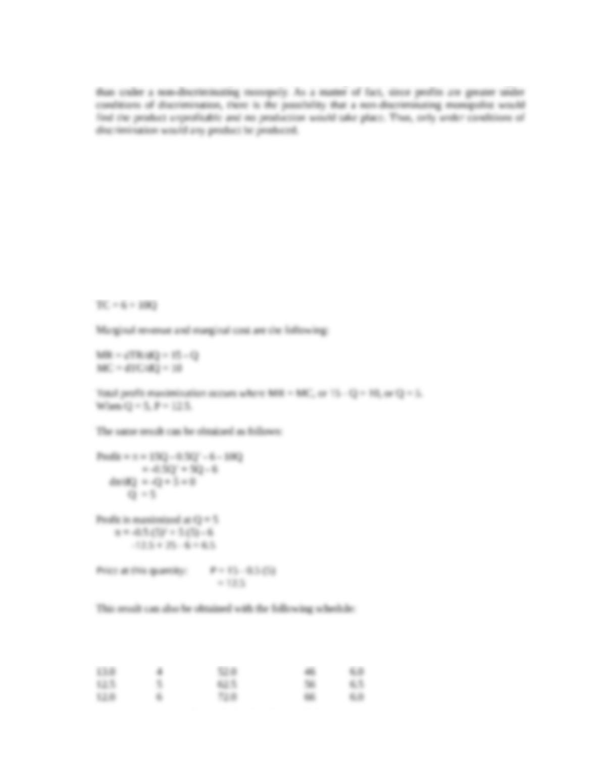
Under certain circumstances, production under third-degree discrimination could also be higher
PROBLEMS
1. The total revenue function is:
Q = 30 – 2P
P = 15 – 0.5Q
TR = Q x P = 15Q – 0.5Q2
The total cost function for the two companies combined is:
Price Quantity Total Revenue Total Cost Profit
15.0 0
14.0 2 28.0 26 2.0
Copyright © 2014 Pearson Education, Inc.
Special Pricing Practices 101
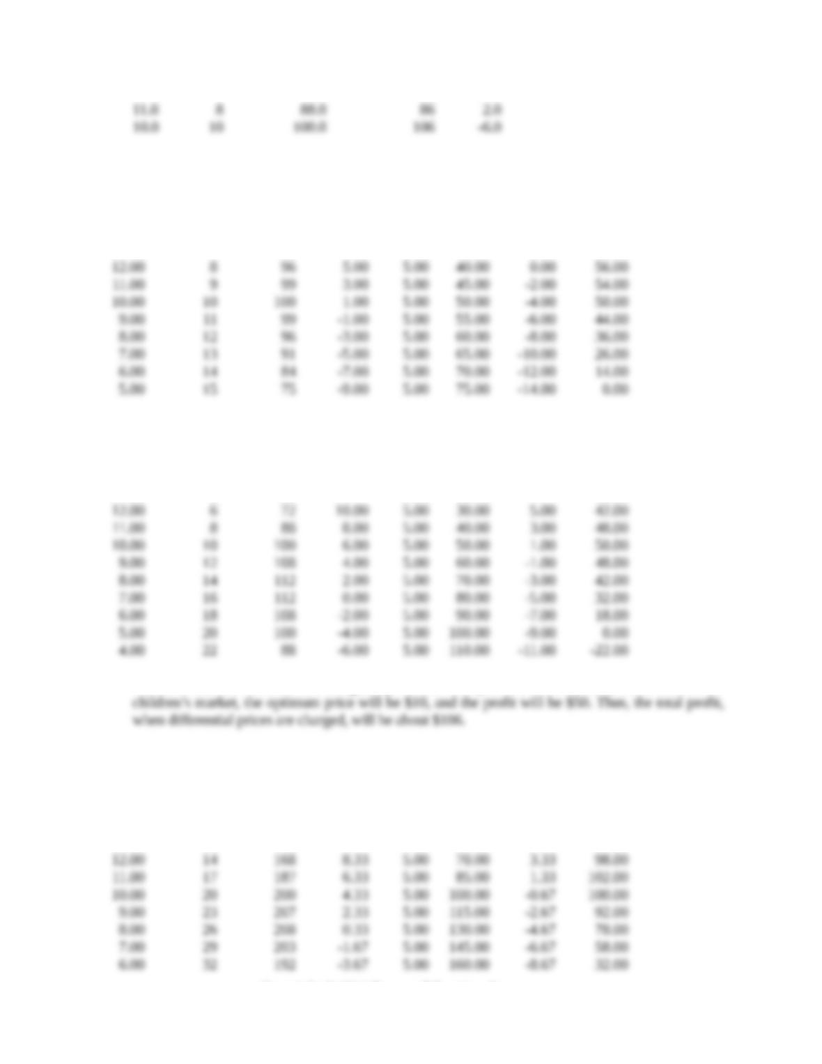
2. a. (1) ADULT MARKET
Total Marginal Marginal Total
Price Quantity Revenue Revenue Cost Cost MR-MC Profit
14.00 6 84 5.00 30.00 54.00
13.00 7 91 7.00 5.00 35.00 2.00 56.00
(2) CHILDREN’S MARKET
Total Marginal Marginal Total
Price Quantity Revenue Revenue Cost Cost MR-MC Profit
13.00 4 52 5.00 20.00 32.00
The adult market will achieve its highest profit between prices of $12 and $13, about $56. In the
(2) COMBINED MARKET
Total Marginal Marginal Total
Price Quantity Revenue Revenue Cost Cost MR-MC Profit
13.00 11 143 5.00 55.00 88.00
Copyright © 2014 Pearson Education, Inc.
Special Pricing Practices 102
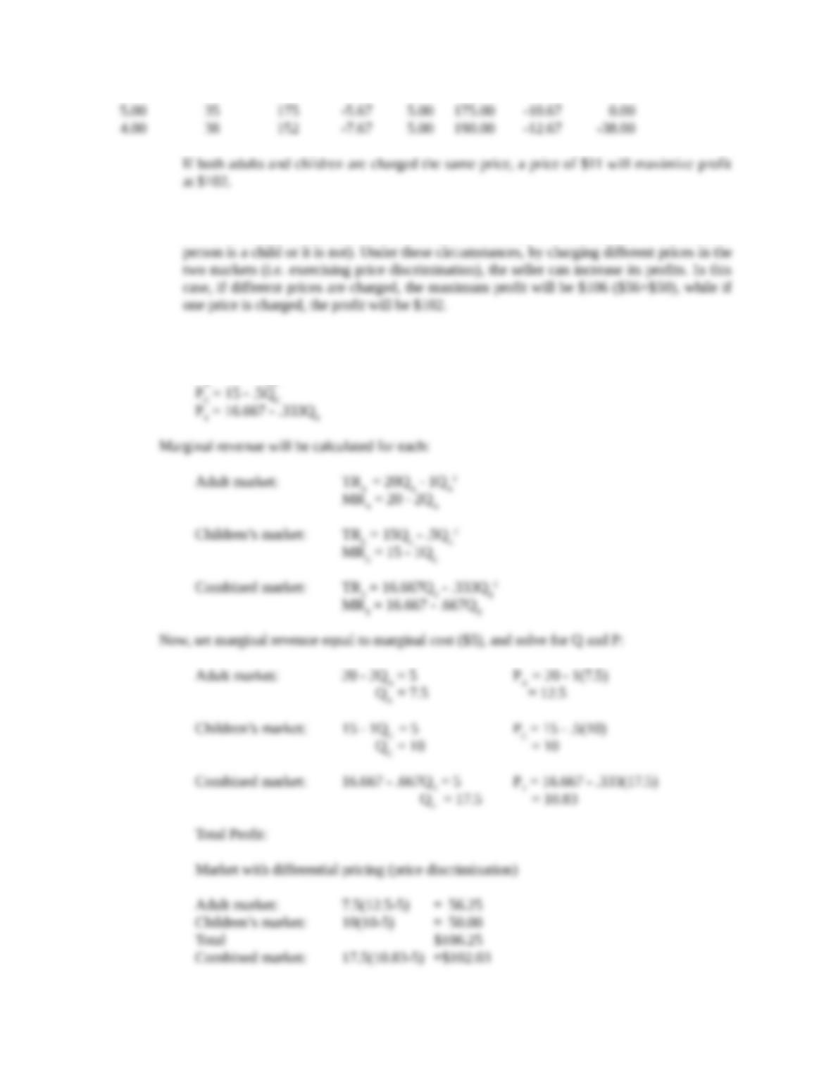
(3) This is a case of third-degree price discrimination. The elasticities of the two demand
curves are different and there are no transfers between the two markets (either the admitted
b. First, each of the demand curves is converted, so that price is the independent variables:
PA = 20 – 1QA
Copyright © 2014 Pearson Education, Inc.
Special Pricing Practices 103
As can be seen, the results are almost exactly the same as in a. The results are mathematically
more precise when equations are used.
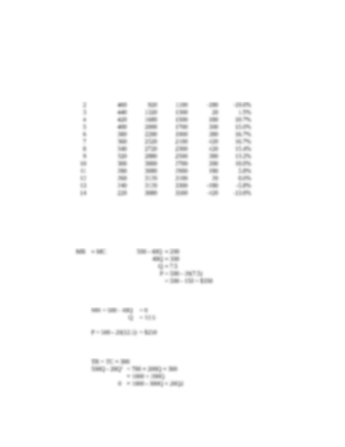
3. a. Total Total Total Profit
Quantity Price Revenue Cost Profit Margin
0 500 0 700 -700
1 480 480 900 -420 -87.5%
(1) Quantity will be between 7 and 8, and price between $340 and $360.
P = 500 – 20Q TC = 700 + 200Q
TR = 500Q – 20Q2MC = 200
MR = 500 – 40Q
(2) Quantity will be between 12 and 13, and price will be between $240 and 260.
(3) Quantity will be 10 and price will be $300.
Solving the above quadratic equation will give Q = 10 and Q = 5. At a quantity of 5,
revenue will be $2000. At a quantity of 10, revenue will be $3000. Profit will be $300 at
Copyright © 2014 Pearson Education, Inc.
Special Pricing Practices 104
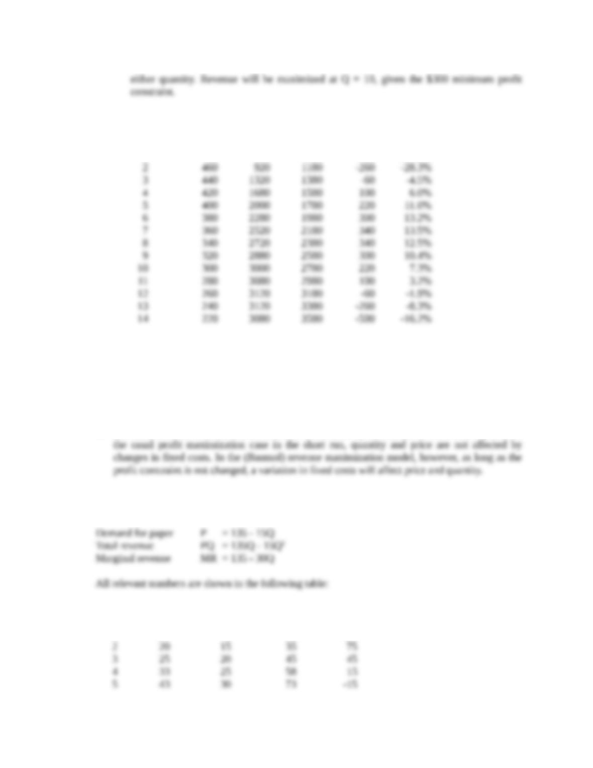
b. Total Total Total Profit
Quantity Price Revenue Cost Profit Margin
0 500 0 780 -780
1 480 480 980 -500 -104.2%
(1) Profit will be maximized at quantity between 7 and 8, and price between $340 and $360.
(2) Revenue will be maximized at quantity between 12 and 13 and price between $240 and
$260.
(3) Quantity will be 9 and price will be $320.
c. The difference between the results in a. and b. is caused by an increase in fixed costs by $80. In
4. The marginal cost of paper is the sum of the marginal cost of pulp plus the marginal cost of
conversion. The marginal revenue is calculated as follows:
MC MC MC MR
Quantity of Pulp of Converting of Paper of Paper
1 18 10 28 105
Copyright © 2014 Pearson Education, Inc.
Special Pricing Practices 105
5. It can be assumed that the $30 purchase cost per pair is constant. In such a case the following
formula can be used to arrive at price:
Ep-1.8
6. If 100 aircraft will be produced:
Fixed cost $ 50,000,000
7. When TC = $15,000, profit = $21,000, strawberries = 1,800 flats, melons = 1,200 cartons.
8. The variable cost per desk for the present situation is:
Copyright © 2014 Pearson Education, Inc.
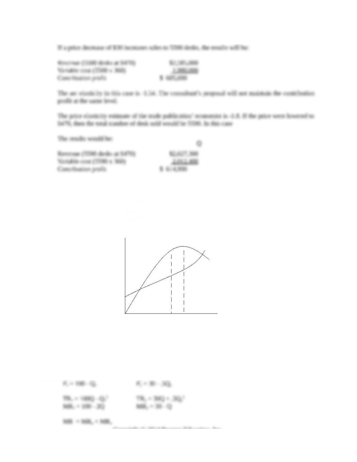
Q
Cost
Revenue
Qp Qs
$
Special Pricing Practices 106
Even with this higher elasticity, the profit contribution would not be maintained.
9. The authors would favor the highest possible revenue. The highest revenue would take place at a
price lower than if profits were maximized. Thus students would be on the side of the authors.
Figure 10.1
Since the demand curve has a negative slope, the unit price will be lower at Qs (where revenue is
maximized) than at Qp (where profit is maximized).
10. a. Qx = 100 – PxQy = 60 – 2Py
Copyright © 2014 Pearson Education, Inc.
Special Pricing Practices 107
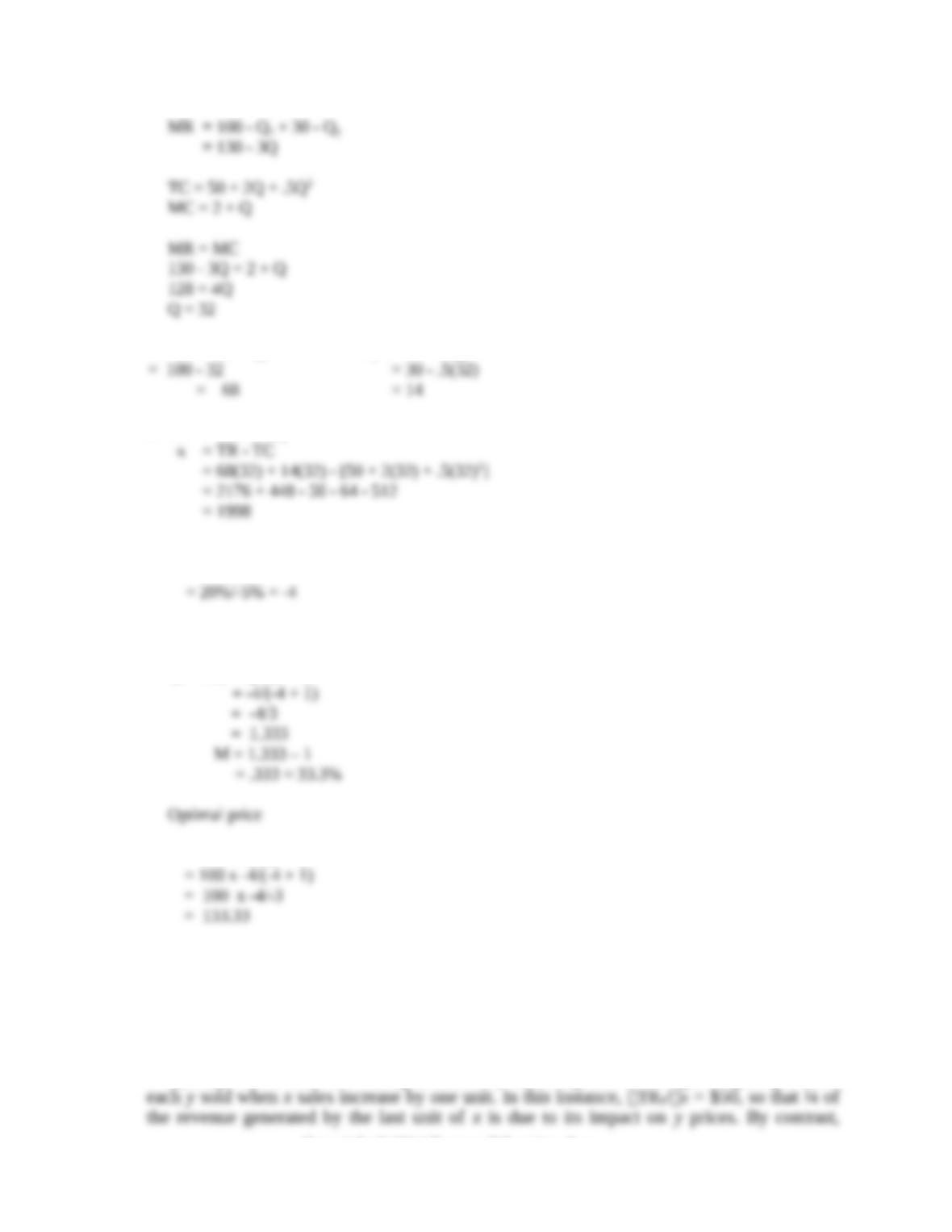
b. Px= 100 – QxPy= 30 – .5Qy
c. TR = TRx + TRy
11. a. εp = %ΔOutput/%Price
b. Optimal markup
(1 + M) = εp/(εp + 1)
P = MC x εp/(εp + 1)
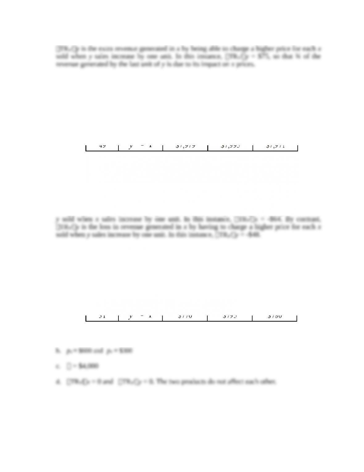
12. a. (x*,y*) = (25, 50)
b. pX = $650 and pY = $275
c. = $8,000
d. TRY/x is the extra revenue generated in y by being able to charge a higher price for
Copyright © 2014 Pearson Education, Inc.
Special Pricing Practices 108
e.
13. a. (x*,y*) = (16, 32)
b. pX = $584 and pY = $308
c. = $800
d. TRY/x is the loss in revenue generated in y by having to charge a lower price for each
e.
14. a. (x*,y*) = (20, 40)
e.
Copyright © 2014 Pearson Education, Inc.
Special Pricing Practices 109
15. As the cross-product effect went from negative to zero to positive, the profit maximizing production
Copyright © 2014 Pearson Education, Inc.