1
O N L I N E T U T O R I A L
Statistical Tools for Managers
1. A probability distribution is a statement of a probability function
which assigns all the probabilities associated with a random variable.
A discrete probability distribution is a distribution of discrete
random variables (i.e., random variable with a limited set of values.)
2. The expected value is the average of the distribution and is
computed for a discrete distribution using the following formula:
3. The variance is a measure of the dispersion of the distribution.
The variance of a discrete probability distribution is given by the
following formula:
4. Examples of business processes which might be described by
a normal distribution could include sales of a product, project
completion time, average weight of a product, and product de-
T1.1
Number of Loaves
Probability
Expected Loaves
0
0.05
0.00
1
0.15
0.15
2
0.20
0.40
3
0.25
0.75
4
0.20
0.80
5
0.15
0.75
p(xi) = 1.00
ni p(xi) = 2.85
The average (expected value) number of loaves is given by:
nave =
ni pi
The store will sell, on average, 2.85 loaves of bread.
Expected value = 5.45
ii
X = X p =
2
Variance = ( ) 4.06
ii
X X p − =
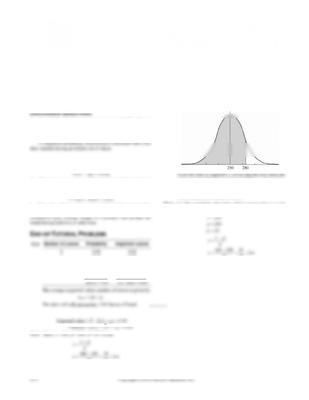
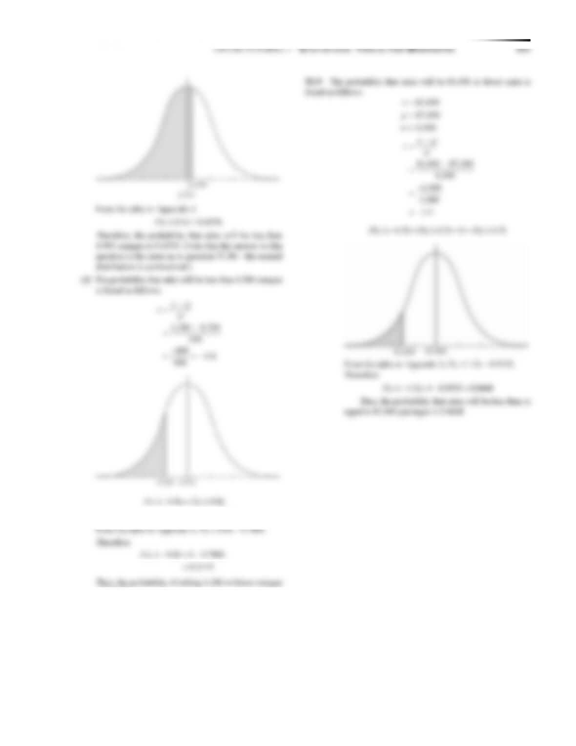
curve corresponding to a z of 1.2 is 0.8849, i.e., P(z 1.2) =
0.8849.
Therefore, the probability that the sales will be less
than or equal to 280 boats is 0.8849.
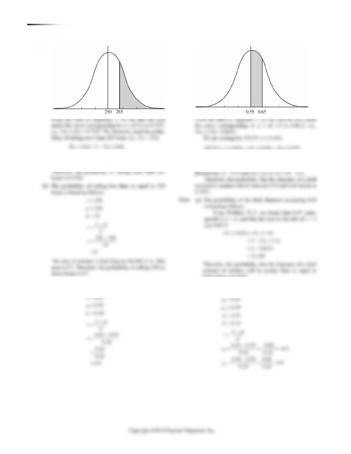
T1.4 (a) The probability that sales will be greater than or equal
to 265 boats is found as follows:
=
−
=
−
= = =
265
265 250 15 0.6
25 25
x
x
z
z
348 ONLINE TUTORIAL 1 STAT IST IC AL TOO L S F O R MANAGERS
350 ONLINE TUTORIAL 1 STAT IST IC AL TOO L S F O R MANAGERS
1
2
1
1
2
2
470
460
450
25
470 450 20
25 25
0.8
460 450 10
25 25
0.4
x
x
x
z
z
z
z
z
=
=
=
=
−
=
−
==
=
−
==
=
Therefore:
= − (460 470) ( 0.8) ( 0.4)P x P z P z
From the table in Appendix I:
=
=
( 0.8) 0.7881
( 0.4) 0.6554
Pz
Pz
and
= − =(460 470) 0.7881 0.6554 0.1327Px
Thus, the probability that the oven temperature will be
between 460 and 470 is 0.1327.
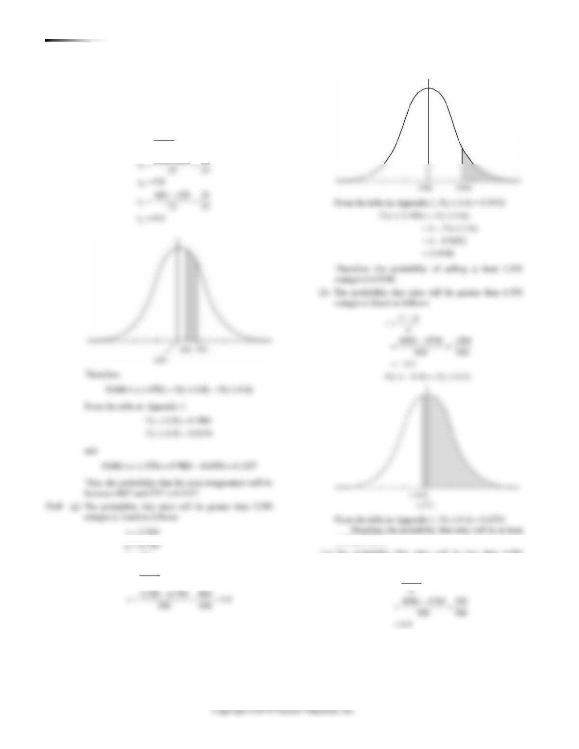
T1.8 (a) The probability that sales will be greater than 5,500
oranges is found as follows:
5,500
4,700
500
5,500 4,700 800 1.6
500 500
x
x
z
z
=
=
=
−
=
−
= = =
From the table in Appendix I, P(z 1.6) = 0.9452.
( 5,500) ( 1.6)
1 ( 1.6)
1 0.9452
0.0548
P x P z
Pz
=
= −
=−
=
Therefore, the probability of selling at least 5,500
oranges is 0.0548.
(b) The probability that sales will be greater than 4,500
oranges is found as follows:
−
=
−−
==
=−
− =
4500 4700 200
500 500
0.4
( 0.4) ( 0.4)
x
z
P z P z
From the table in Appendix I, P(z 0.4) = 0.6554
Therefore, the probability that sales will be at least
4500 is 0.6554.
(c) The probability that sales will be less than 4,900
oranges is found as follows:
−
=
−
==
=
4900 4700 200
500 500
0.4
x
z
4,900 oranges is 0.6554. (Note that the answer to this
question is the same as to question T1.8b—the normal
distribution is symmetrical.)
4,300 4,700
500
400 0.8
500
x
z
−
=
−
=
−
= = −
− =
= −
( 0.8) ( 0.8)
1 ( 0.8)
P z P z
Pz
From the table in Appendix I, P(z 1.5) = 0.9332.
Therefore:
− = − =( 1.5) 1 0.9332 0.0668Pz
Thus, the probability that sales will be less than or
equal to 81,000 packages is 0.0668.
348 ONLINE TUTORIAL 1 STAT IST IC AL TOO L S F O R MANAGERS
350 ONLINE TUTORIAL 1 STAT IST IC AL TOO L S F O R MANAGERS
1
2
1
1
2
2
470
460
450
25
470 450 20
25 25
0.8
460 450 10
25 25
0.4
x
x
x
z
z
z
z
z
=
=
=
=
−
=
−
==
=
−
==
=
Therefore:
= − (460 470) ( 0.8) ( 0.4)P x P z P z
From the table in Appendix I:
=
=
( 0.8) 0.7881
( 0.4) 0.6554
Pz
Pz
and
= − =(460 470) 0.7881 0.6554 0.1327Px
Thus, the probability that the oven temperature will be
between 460 and 470 is 0.1327.
T1.8 (a) The probability that sales will be greater than 5,500
oranges is found as follows:
5,500
4,700
500
5,500 4,700 800 1.6
500 500
x
x
z
z
=
=
=
−
=
−
= = =
From the table in Appendix I, P(z 1.6) = 0.9452.
( 5,500) ( 1.6)
1 ( 1.6)
1 0.9452
0.0548
P x P z
Pz
=
= −
=−
=
Therefore, the probability of selling at least 5,500
oranges is 0.0548.
(b) The probability that sales will be greater than 4,500
oranges is found as follows:
−
=
−−
==
=−
− =
4500 4700 200
500 500
0.4
( 0.4) ( 0.4)
x
z
P z P z
From the table in Appendix I, P(z 0.4) = 0.6554
Therefore, the probability that sales will be at least
4500 is 0.6554.
(c) The probability that sales will be less than 4,900
oranges is found as follows:
−
=
−
==
=
4900 4700 200
500 500
0.4
x
z
4,900 oranges is 0.6554. (Note that the answer to this
question is the same as to question T1.8b—the normal
distribution is symmetrical.)
4,300 4,700
500
400 0.8
500
x
z
−
=
−
=
−
= = −
− =
= −
( 0.8) ( 0.8)
1 ( 0.8)
P z P z
Pz
From the table in Appendix I, P(z 1.5) = 0.9332.
Therefore:
− = − =( 1.5) 1 0.9332 0.0668Pz
Thus, the probability that sales will be less than or
equal to 81,000 packages is 0.0668.