F
B U S I N E S S A N A L Y T I C S M O D U L E
1. The seven steps of simulation are define the problem;
introduce the important variables associated with the problem;
construct a numerical model; set up possible courses of action for
3. It allows for the inclusion of real-world complications that
most models cannot permit.
4. It allows “time compression.”
5. It allows the user to ask “what-if” questions and
experiment with various representations of the problem.
6. It does not interfere with the real world system.
7. It allows us to study interactive effects of individual
components or variables.
2. It does not generate optimal solutions to problems.
3. Managers must generate all of the conditions and constraints
for solutions that they want to examine.
4. Each solution model is unique. Its solutions and inferences
are usually not transferable to other problems.
constructed, is affected by the number of trials or repetitions, and is
affected by the random numbers selected. For small numbers of
repetitions, simulated average demand can be quite variable.
5. The role of random numbers in simulation is to help generate
outcomes for random variables. Each random number represents a
particular possibility.
6. Results of a simulation differ from run to run because differ-
numbers to develop values for random variables described by
appropriate probability distributions:
The steps in developing a Monte Carlo simulation are:
◼ Step 1: Establish a probability distribution for each random
8. Simulation can be used in business in dozens of ways, from
examining lines in banks and post offices, to testing inventory
policies, to layout of a plant, to scheduling employees and parts,
9. Simulation is widely used because complex real-world sys-
tems can be examined and tested without impacting on the actual
situation. It also allows for “time–compression,” allows “what-if”
10. Special-purpose languages have these advantages:
(1) They require less programming time for large simulations.
(2) They are usually more efficient and easier to check for
errors.
11. A computer is necessary for three reasons:
◼ It can perform the individual trials in much less time than
12. Inventory ordering policy:
◼ May require simulation if lead time and daily demand are
not constant. Also useful if data do not follow a traditional
probability distribution.
332 BUSINESS ANALYTICS MODULE F SI M U L A T I ON
or if other queuing model assumptions are violated (for
example, if FIFO is not observed).
Bank teller service windows:
5
6
0.15
11–25
6
0.25
26–50
7
0.30
51–80
8
0.20
F.6
At t = 0
RN = 07 so 0 arrivals
At t = 1
RN = 60 so 1 arrival
Server
RN = 77 and it takes 3 minutes to serve
At t = 2
RN = 49 so 1 arrival
Server
RN = 76 so it takes 3 minutes to serve
5
6
0.15
11–25
6
0.25
26–50
7
0.30
51–80
8
0.20
F.6
At t = 0
RN = 07 so 0 arrivals
At t = 1
RN = 60 so 1 arrival
Server
RN = 77 and it takes 3 minutes to serve
At t = 2
RN = 49 so 1 arrival
Server
RN = 76 so it takes 3 minutes to serve
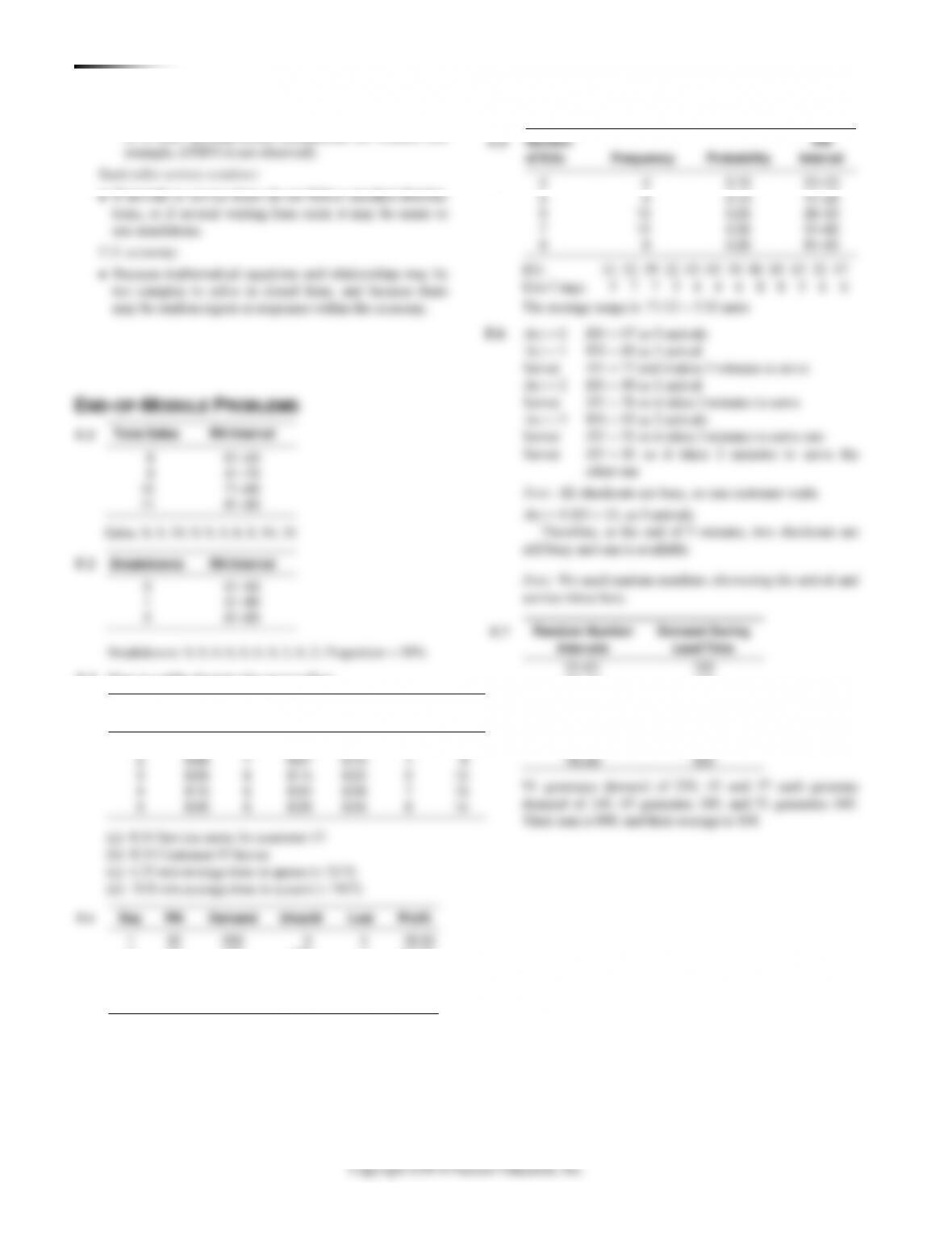
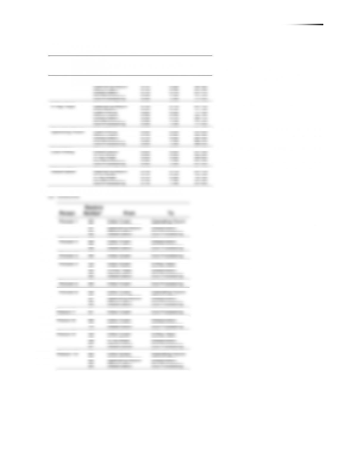
F.1
Tuna Sales
RN Interval
8
01–40
9
41–70
10
71–90
11
91–00
Sales: 8, 9, 10, 9, 9, 9, 8, 8, 10, 10
F.2
Breakdowns
RN Interval
0
01–50
1
51–80
2
81–00
Breakdowns: 0, 0, 0, 0, 0, 0, 0, 2, 0, 2; Proportion = 20%
Day
Demand
Unsold
Profit
1
0
0
20.00
2
100
0
3
0
0
20.00
4
0
17.50
20.00
76–00
220
2
8:06
7
8:07
8:14
1
8
3
8:09
8
8:14
8:22
5
4
8:15
6
8:22
8:28
7
Day
Demand
Unsold
Profit
1
0
0
20.00
2
100
0
3
0
0
20.00
4
0
17.50
20.00
76–00
220
2
8:06
7
8:07
8:14
1
8
3
8:09
8
8:14
8:22
5
4
8:15
6
8:22
8:28
7
F.5
Number
RN
of Kits
Frequency
Probability
Interval
4
4
0.10
01–10
At t = 3
RN = 95 so 2 arrivals
Server
RN = 51 so it takes 3 minutes to serve one
Server
RN = 16 so it takes 2 minutes to serve the
other one
Note: All checkouts are busy, so one customer waits.
At t = 4 RN = 14, so 0 arrivals
Therefore, at the end of 5 minutes, two checkouts are
still busy and one is available.
Note: We used random numbers alternating for arrival and
service times here.
F.7
Random Number
Demand During
Intervals
Lead Time
01–01
100
02–16
120
17–46
140
47–61
160
62–65
180
66–75
200
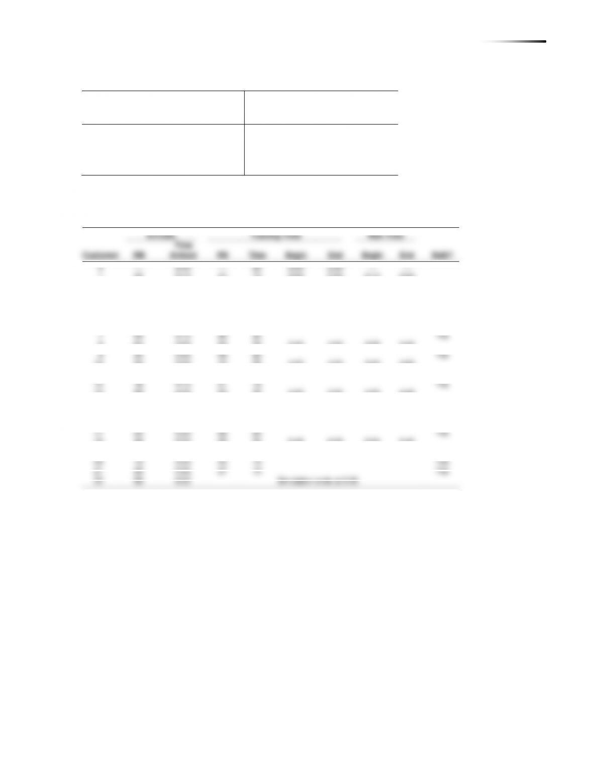
F.3
Here is a table showing the service flow:
Customer
Arrival
Service
Service
Service
Time in
Time in
Number
Time
Time
Begins
Ends
Line
System
1
8:01
6
8:01
8:07
0
6
BUSINESS ANALYTICS MODULE F SI M U L A T I O N 333
1
2
3
4
1
2
3
4
11:09.
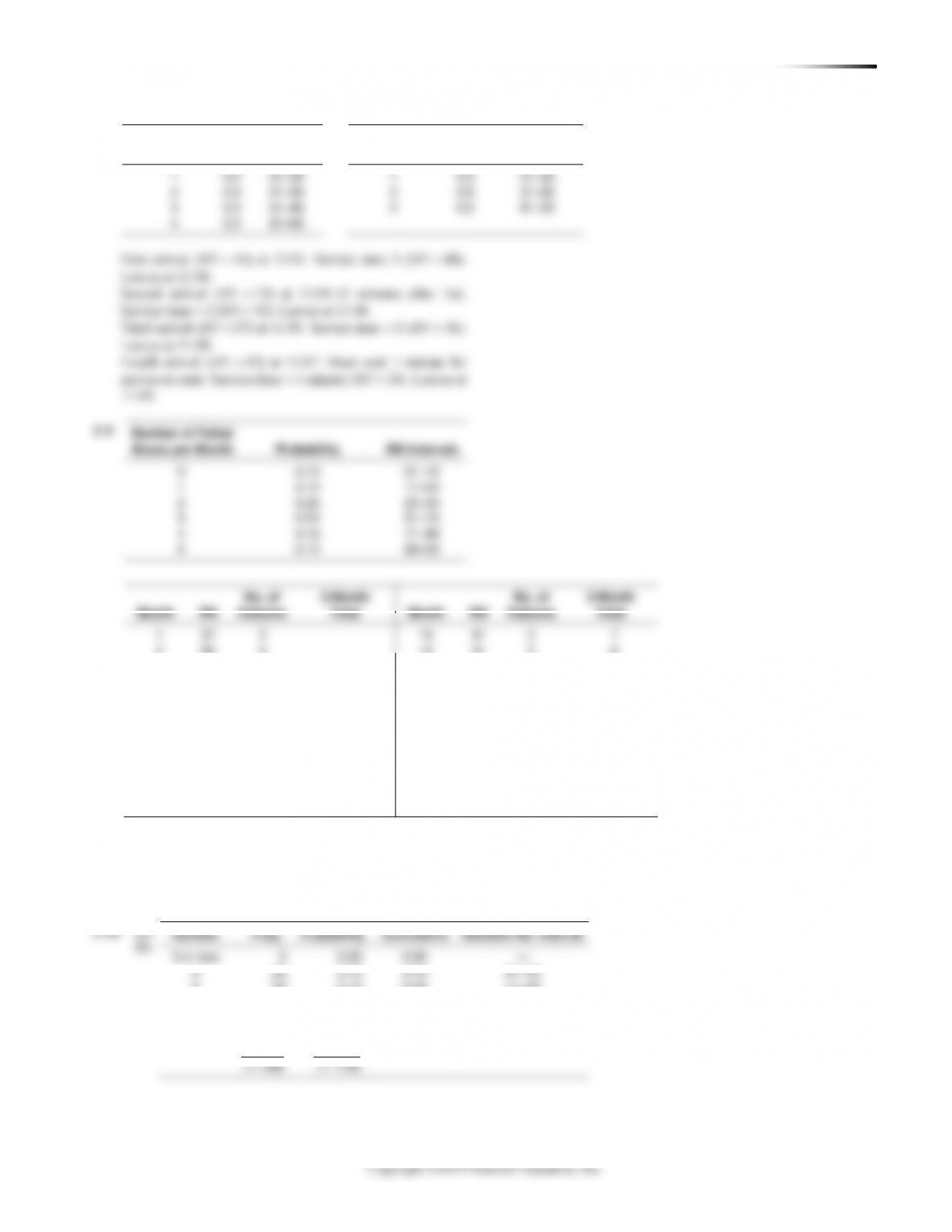
F.9
Number of Failed
Boxes per Month
Probability
RN Intervals
0
0.10
01–10
1
0.14
11–24
2
0.26
25–50
3
0.20
51–70
4
0.18
71–88
5
0.12
89–00
Number
Probability
Cumulative
Number
Probability
Cumulative
F.8
Time Between
Arrivals
Prob.
RN Interval
Service Time
Prob.
RN Interval
No. of
3-Month
No. of
3-Month
Month
RN
Failures
Total
Month
RN
Failures
Total
334 BUSINESS ANALYTICS MODULE F SI M U L A T I ON
(c)
Hour
Random*
Arrivals
1
52
7
2
37
6
3
82
8
4
69
7
5
98
8
6
96
8
7
33
6
8
50
6
9
88
8
10
90
8
11
50
6
12
27
6
13
45
6
14
81
8
15
66
7
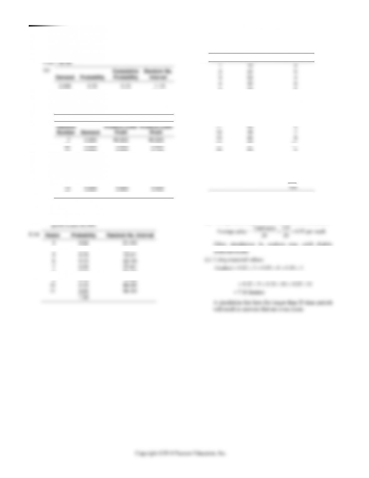
= 105
105
Average number of arrivals per hour = = 7 cars
15
F.11 (a) Day 3 demand = 24
(b) Net profit total = $36.70
(c) Lost goodwill on day 6 = $.30
0.10
37
19
52
22
0.10
37
19
52
22
336 BUSINESS ANALYTICS MODULE F SI M U L A T I ON
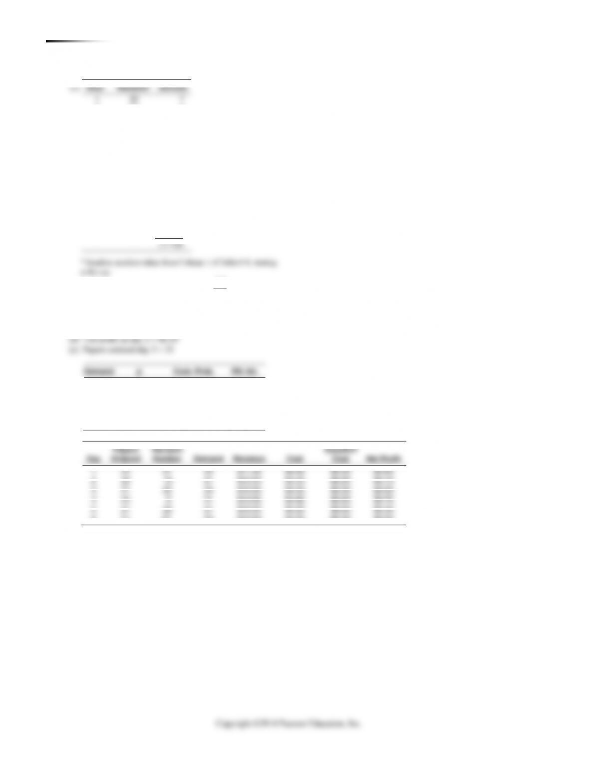
F.13
Selling price = $2
Cost = $0.80
(a)
Cumulative
Random No.
Demand
Probability
Probability
Interval
2,300
0.15
0.15
1–15
2,400
0.22
0.37
16–37
2,500
0.24
0.61
38–61
2,600
0.21
0.82
62–82
2,700
0.18
1.00
83–00
Random
Produce 2,500
Produce 2,600
Number
Demand
Profit
Profit
7
2,300
$2,600
$2,520
60
2,500
3,000
2,920
77
2,600
3,000
3,120
49
2,500
3,000
2,920
76
2,600
3,000
3,120
95
2,700
3,000
3,120
51
2,500
3,000
2,920
16
2,400
2,800
2,720
14
2,300
2,600
2,520
85
2,700
3,000
3,120
(b) If the company produces 2,500 programs, the average
profit is $2,900.
(c) If the company produces 2,600 programs, the average
Heater
Random No. Interval
3
4
5
6
7
8
9
1.00
Heater
Random No. Interval
3
4
5
6
7
8
9
1.00
(a)
Week
Random
Simulated Sales
1
10
4
2
24
6
3
03
4
4
32
6
5
23
6
6
59
7
7
95
10
8
34
6
9
34
6
10
51
7
11
08
4
12
48
7
13
66
8
14
97
11
15
03
4
16
96
11
17
46
7
18
74
9
19
77
9
20
44
7
139
With a supply of 8 heaters, Higgins will stock
out 5 times during the 20-week period (in weeks
7, 14, 16, 18, and 19).
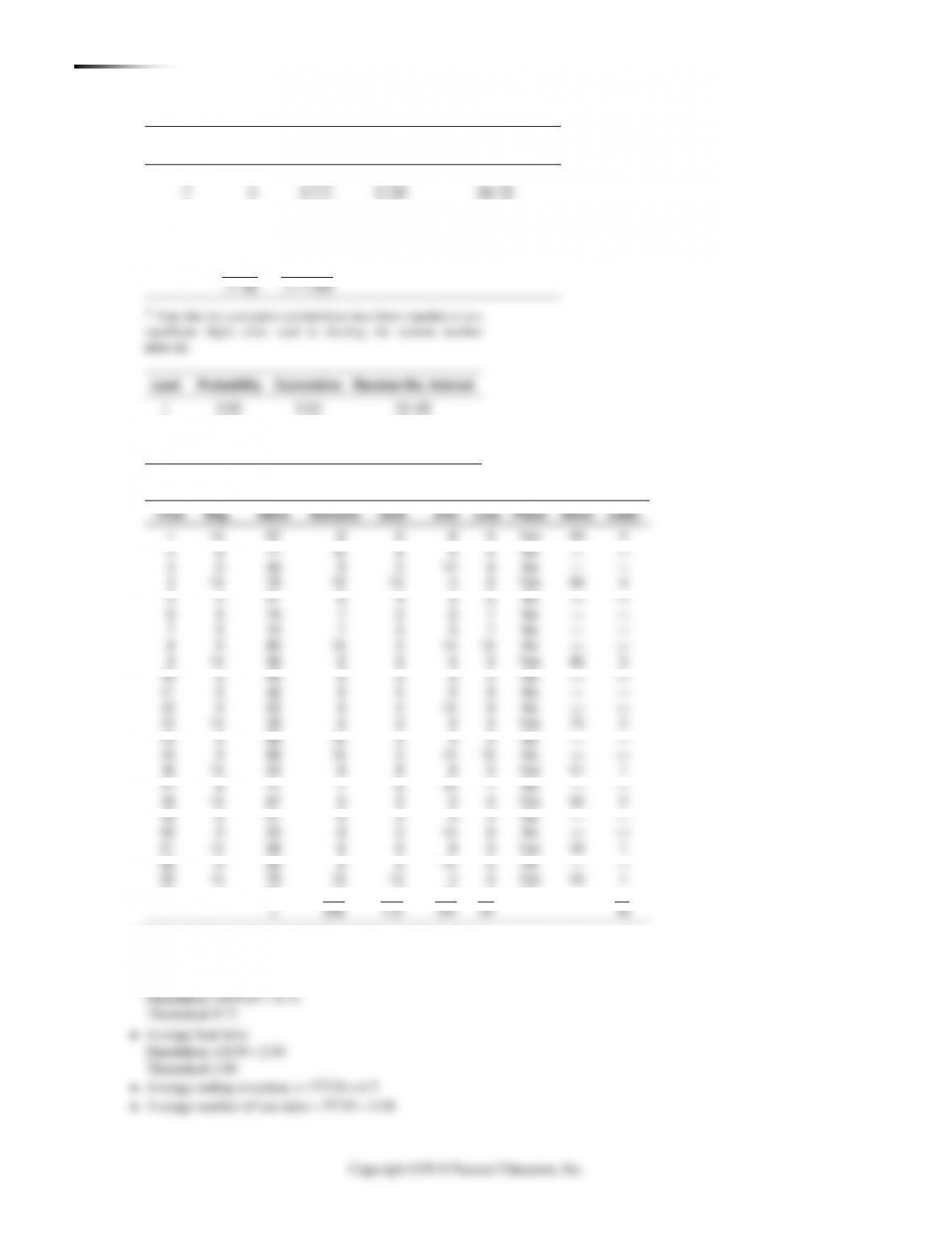
(b) Average sales as given by the results of the simulation:
was 105 minutes. This equates to 105/10 $2.00, or $21.00
per day. This translates to $504 per month. The addition of
another tanning bed (at $600/month) is not justified.
338 BUSINESS ANALYTICS MODULE F SI M U L A T I ON
7
4
0.111
0.194
09–19
8
6
0.167
0.361
20–36
9
12
0.333
0.694
37–69
9
0.250
0.944
70–94
1
0.028
0.972
95–97
1
0.028
1.000
98–00
0.44
0.33
0.16
Place
Rand
2
4
3
2
1
2
1
1
7
4
0.111
0.194
09–19
8
6
0.167
0.361
20–36
9
12
0.333
0.694
37–69
9
0.250
0.944
70–94
1
0.028
0.972
95–97
1
0.028
1.000
98–00
0.44
0.33
0.16
Place
Rand
2
4
3
2
1
2
1
1
F.16 (a)
Demand for
Cumulative
Random Number
Mercedes
Freq.
Probability
Probability
Interval*
6
3
0.083
0.083
01–08
520,710
= $520,110, or $21,671 per month
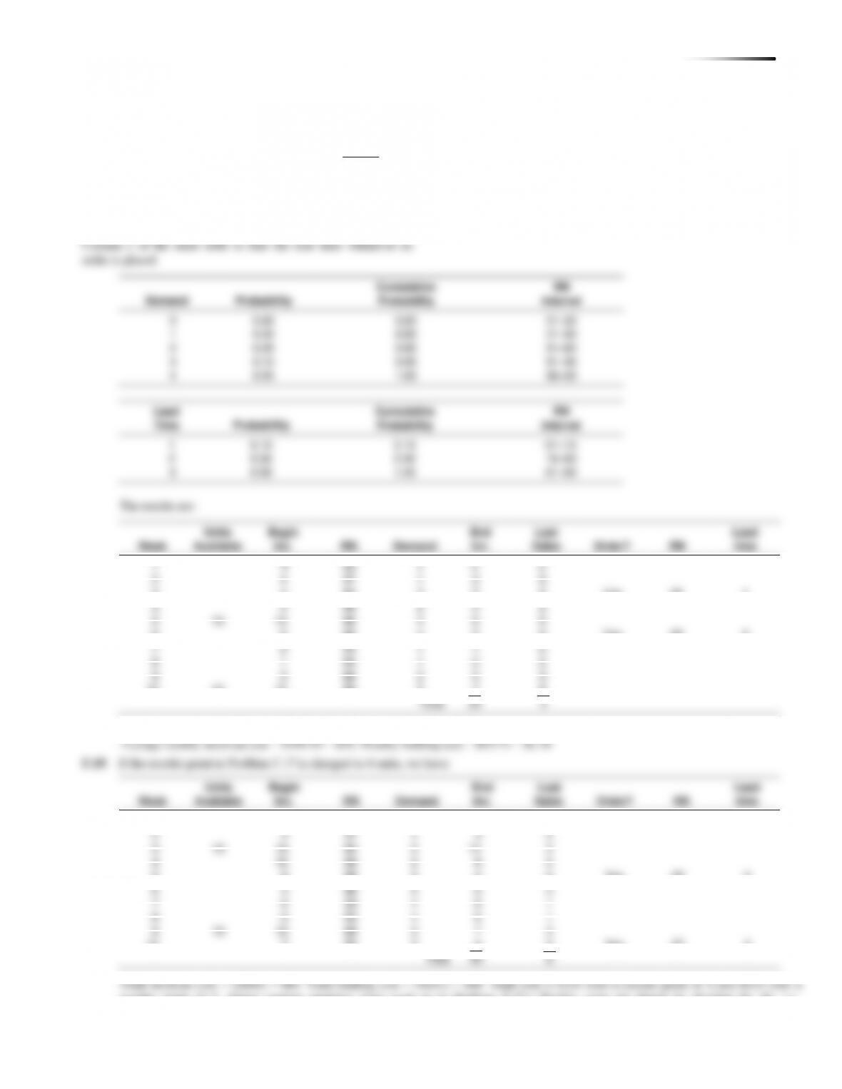
F.17 We use the following random number intervals when
simulating demand and lead time. We then select Column 1 of
text Table F.4 to get the random numbers for demand, and use
332 BUSINESS ANALYTICS MODULE F SI M U L A T I ON
or if other queuing model assumptions are violated (for
example, if FIFO is not observed).
Bank teller service windows:
F.1
Tuna Sales
RN Interval
8
01–40
9
41–70
10
71–90
11
91–00
Sales: 8, 9, 10, 9, 9, 9, 8, 8, 10, 10
F.2
Breakdowns
RN Interval
0
01–50
1
51–80
2
81–00
Breakdowns: 0, 0, 0, 0, 0, 0, 0, 2, 0, 2; Proportion = 20%
F.5
Number
RN
of Kits
Frequency
Probability
Interval
4
4
0.10
01–10
At t = 3
RN = 95 so 2 arrivals
Server
RN = 51 so it takes 3 minutes to serve one
Server
RN = 16 so it takes 2 minutes to serve the
other one
Note: All checkouts are busy, so one customer waits.
At t = 4 RN = 14, so 0 arrivals
Therefore, at the end of 5 minutes, two checkouts are
still busy and one is available.
Note: We used random numbers alternating for arrival and
service times here.
F.7
Random Number
Demand During
Intervals
Lead Time
01–01
100
02–16
120
17–46
140
47–61
160
62–65
180
66–75
200
F.3
Here is a table showing the service flow:
Customer
Arrival
Service
Service
Service
Time in
Time in
Number
Time
Time
Begins
Ends
Line
System
1
8:01
6
8:01
8:07
0
6
BUSINESS ANALYTICS MODULE F SI M U L A T I O N 333
11:09.
F.9
Number of Failed
Boxes per Month
Probability
RN Intervals
0
0.10
01–10
1
0.14
11–24
2
0.26
25–50
3
0.20
51–70
4
0.18
71–88
5
0.12
89–00
F.8
Time Between
Arrivals
Prob.
RN Interval
Service Time
Prob.
RN Interval
No. of
3-Month
No. of
3-Month
Month
RN
Failures
Total
Month
RN
Failures
Total
334 BUSINESS ANALYTICS MODULE F SI M U L A T I ON
(c)
Hour
Random*
Arrivals
1
52
7
2
37
6
3
82
8
4
69
7
5
98
8
6
96
8
7
33
6
8
50
6
9
88
8
10
90
8
11
50
6
12
27
6
13
45
6
14
81
8
15
66
7
= 105
105
Average number of arrivals per hour = = 7 cars
15
F.11 (a) Day 3 demand = 24
(b) Net profit total = $36.70
(c) Lost goodwill on day 6 = $.30
336 BUSINESS ANALYTICS MODULE F SI M U L A T I ON
F.13
Selling price = $2
Cost = $0.80
(a)
Cumulative
Random No.
Demand
Probability
Probability
Interval
2,300
0.15
0.15
1–15
2,400
0.22
0.37
16–37
2,500
0.24
0.61
38–61
2,600
0.21
0.82
62–82
2,700
0.18
1.00
83–00
Random
Produce 2,500
Produce 2,600
Number
Demand
Profit
Profit
7
2,300
$2,600
$2,520
60
2,500
3,000
2,920
77
2,600
3,000
3,120
49
2,500
3,000
2,920
76
2,600
3,000
3,120
95
2,700
3,000
3,120
51
2,500
3,000
2,920
16
2,400
2,800
2,720
14
2,300
2,600
2,520
85
2,700
3,000
3,120
(b) If the company produces 2,500 programs, the average
profit is $2,900.
(c) If the company produces 2,600 programs, the average
(a)
Week
Random
Simulated Sales
1
10
4
2
24
6
3
03
4
4
32
6
5
23
6
6
59
7
7
95
10
8
34
6
9
34
6
10
51
7
11
08
4
12
48
7
13
66
8
14
97
11
15
03
4
16
96
11
17
46
7
18
74
9
19
77
9
20
44
7
139
With a supply of 8 heaters, Higgins will stock
out 5 times during the 20-week period (in weeks
7, 14, 16, 18, and 19).
(b) Average sales as given by the results of the simulation:
was 105 minutes. This equates to 105/10 $2.00, or $21.00
per day. This translates to $504 per month. The addition of
another tanning bed (at $600/month) is not justified.
338 BUSINESS ANALYTICS MODULE F SI M U L A T I ON
F.16 (a)
Demand for
Cumulative
Random Number
Mercedes
Freq.
Probability
Probability
Interval*
6
3
0.083
0.083
01–08
520,710
= $520,110, or $21,671 per month
F.17 We use the following random number intervals when
simulating demand and lead time. We then select Column 1 of
text Table F.4 to get the random numbers for demand, and use