88 SUPPLEMENT 6 ST A T I S T I C A L PR O C E S S CO N T R O L
Sample
in Sample
of Late Flights
1
2
3
4
5
6
7
8
9
10
11
12
13
14
S6.33
( )( )( – ) (.04)(.57)(500 – 60) 10.0
AOQ = .02
500 500
AOQ 2.0%
da
P P N n
N= = =
=
S6.34
(a)
X
Range
Upper control limit
61.131
41.62
Center line (avg)
49.776
19.68
Lower control limit
38.421
0.00
Recent Data Sample
Hour
1
2
3
4
5
X
R
26
48
52
39
57
61
51.4
22
27
45
53
48
46
66
51.6
21
28
63
49
50
45
53
52.0
18
29
47
70
45
52
61
57.0
25
30
45
38
46
54
52
47.0
16
(b) Yes, the process appears to be under control. Samples
26–30 stayed within the boundaries of the upper and
50 hours, which supports the claim made by West Battery
Corp. However, the variance from the mean needs to be
controlled and reduced. Lifetimes should deviate from the
S6.35
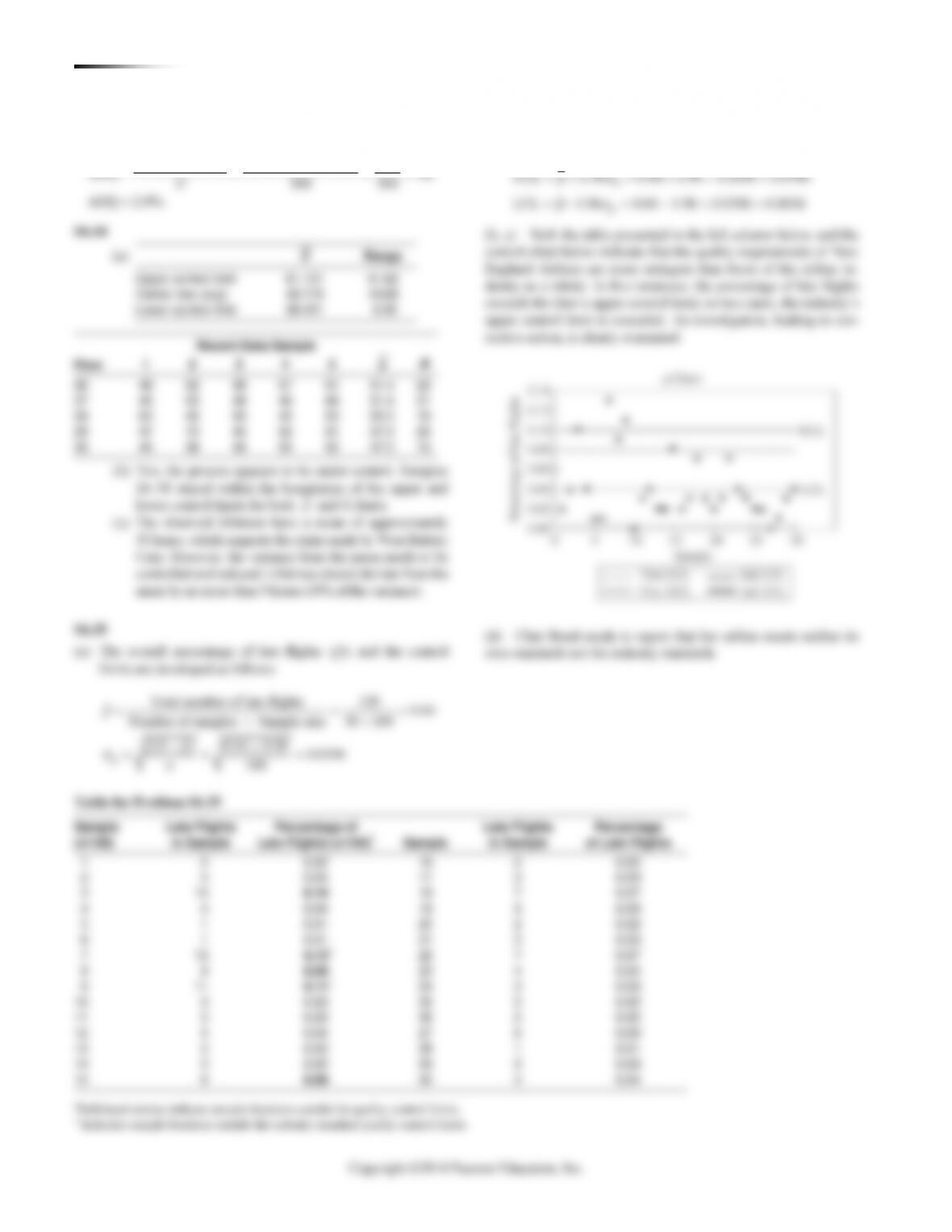
(a) The overall percentage of late flights
and the control
Then the control limits are given (for a 95% confidence inter–
val; 95% = 1.96) by:
UCL 1.96 0.04 1.96 0.0196 0.0784
LCL 1.96 0.04 1.96 0.0196 0.0016
p
p
p
p
= + = + =
= − = − =
(b, c) Both the table presented in the left column below and the
control chart below indicate that the quality requirements of New
England Airlines are more stringent than those of the airline in-
dustry as a whole. In five instances, the percentage of late flights
exceeds the firm’s upper control limit; in two cases, the industry’s
upper control limit is exceeded. An investigation, leading to cor-
rective action, is clearly warranted.
(d) Clair Bond needs to report that her airline meets neither its
1.95
75 3 76.85
10
1.95
75 3 73.15
10
X
X
UCL
LCL
= + =
= − =
S6.37 n = 5. From Table S6.1, A2 = 0.577, D4 = 2.115, D3 = 0
2
2
(a) 50 0.577 4 52.308
50 0.577 4 47.692
X
X
UCL X A R
LCL X A R
= + = + =
= − = − =
4
3
(b) 2.115 4 8.456
0 4 0
R
R
UCL D R
LCL D R
= = =
= = =
S6.38 n = 10. From Table S6.1, A2 = 0.308, D4 = 1.777, D3 = 0.233
2
2
4
3
60 0.308 3 60.924
60 0.308 3 59.076
1.777 3 5.331
0.223 3 0.669
X
X
R
R
UCL X A R
LCL X A R
UCL D R
LCL D R
= + = + =
= − = − =
= = =
= = =
S6.39
Sample
X
R
Sample
X
R
Sample
X
R
1
63.5
2.0
10
63.5
1.3
19
63.8
1.3
2
63.6
1.0
11
63.3
1.8
20
63.5
1.6
3
63.7
1.7
12
63.2
1.0
21
63.9
1.0
4
63.9
0.9
13
63.6
1.8
22
63.2
1.8
5
63.4
1.2
14
63.3
1.5
23
63.3
1.7
6
63.0
1.6
15
63.4
1.7
24
64.0
2.0
7
63.2
1.8
16
63.4
1.4
25
63.4
1.5
8
63.3
1.3
17
63.5
1.1
9
63.7
1.6
18
63.6
1.8
= = =
= = =
2 4 3
63.49, 1.5, 4. From Table S6.1,
0.729, 2.282, 0.0.
X R n
A D D
2
2
4
3
63.49 0.729 1.5 64.58
63.49 0.729 1.5 62.40
2.282 1.5 3.423
0 1.5 0
X
X
R
R
UCL X A R
LCL X A R
UCL D R
LCR D R
= + = + =
= − = − =
= = =
= = =
S6.40
= = = = =
24
19.90, 0.34, 4, 0.729, 2.282X R n A D
()
()
= + =
= − =
(a) 19.90 0.729 0.34 20.15
19.90 0.729 0.34 19.65
X
X
UCL
LCL
()
==
=
(b) 2.282 0.34 0.78
0
R
R
UCL
LCL
S6.41
Desired Desired
3.5, 50, 6R X n= = =
= + = + =
= − = − =
= = =
= = =
2
2
3
4
50 0.483 3.5 51.69
50 0.483 3.5 48.31
2.004 3.5 7.014
0 3.5 0
X
X
R
R
UCL X A R
LCL X A R
UCL D R
LCL D R
The smallest sample range is 1, and the largest 6. Both are
well within the control limits.
The smallest average is 47, and the largest 57. Both are
outside the proper control limits.
Therefore, although the range is with limits, the average is
outside limits, and apparently increasing. Immediate action is
needed to correct the problem and get the average within the
con-trol limits again.
*Note to instructor: To broaden the selection of homework prob-
lems, these additional problems are also available to you and your
students.
90 SUPPLEMENT 6 ST A T I S T I C A L PR O C E S S CO N T R O L
S6.42 0.51
_ _ _ _ _ _ _ _ _ _ _ _ _ _ _ _ _ 0.505 drill bit (largest)
_ _ _ _ _ _ _ _ _ _ _ _ _ _ _ _ _ 0.495 drill bit (smallest)
0.49
0.505 – 0.49 = 0.015, 0.015/0.00017 = 88 holes within
standard
0.495 – 0.49 = 0.005, 0.005/0.00017 = 29 holes within
standard
Any one drill bit should produce at least 29 holes that meet
No.
In Control?
0.105
0.04
0.09
0.07
0.1
0.06
0.145
0.12
0.08
0.1
0.06
0.035
0.065
0.12
0.08
No.
In Control?
0.105
0.04
0.09
0.07
0.1
0.06
0.145
0.12
0.08
0.1
0.06
0.035
0.065
0.12
0.08
S6.45
Number
Number
Number
Day
Defective
Day
Defective
Day
Defective
1
6
8
3
15
4
2
5
9
6
16
5
3
6
10
3
17
6
4
4
11
7
18
5
5
3
12
5
19
4
6
4
13
4
20
3
SUPPLEMENT 6 ST A T I S T I C A L PR O C ES S CO N T R O L 91
19
21
0.105
Y
20
26
0.13
Y
21
28
0.14
Y
22
22
0.11
Y
23
17
0.085
Y
24
14
0.07
Y
25
12
0.06
Y
p-bar = 0.0924
Std. Deviation of p = 0.020477
UCLp = 0.154
LCLp = 0.031
The process is not in control as sample 16 exceeds the UCL.
When sample 16 is removed and the control limits recalculated,
the process is in control, based on the data. This points out the
importance of statistical sampling in process control.
S6.47
Total number of incidents/Total number of residents
156 /10,000 0.0156
(1 ) [(0.0156)(1 0.0156)]/1,000 0.0039
1,000
Upper tolerance
0.403
Process capability
limit
index
Lower tolerance
0.4
Upper one
limit
sided index
Mean
0.401
Lower one
sided index
Standard deviation
0.0004
Upper tolerance limit
Lower tolerance limit
Standard deviation
Standard deviation
Upper tolerance
0.403
Process capability
limit
index
Lower tolerance
0.4
Upper one
limit
sided index
Mean
0.401
Lower one
sided index
Standard deviation
0.0004
Upper tolerance limit
Lower tolerance limit
Standard deviation
Standard deviation
p
p
pp
=
==
−
= = − =
S6.49
Time
Box 1
Box 2
Box 3
Box 4
Average
9 AM
9.8
10.4
9.9
10.3
10.1
10 AM
10.1
10.2
9.9
9.8
10.0
11 AM
9.9
10.5
10.3
10.1
10.2
12 PM
9.7
9.8
10.3
10.2
10.0
1 PM
9.7
10.1
9.9
9.9
9.9
Average=
10.04
Std. Dev. =
0.11
10.1 10 10 9.9
0.3 and 0.3
(3)(0.11) (3)(0.11)
−−
==
As 0.3 is less than 1, the process will not produce within the
specified tolerance.
S6.50 Machine 1 produces “off–center” with a smaller standard
deviation than Machine 2. Machine 1 has index of 0.83, and
Machine 2 has an index of 1.0. Thus, Machine 1 is not capable.
Machine 2 is capable.
92 SUPPLEMENT 6 ST A T I S T I C A L PR O C E S S CO N T R O L
1. The first thing that must be done is to develop quality control
limits for the sample means. This can be done as follows. Because
the process appears to be unstable, we can use the desired mean as
a 99.73% confidence interval Z = 3:
3 50 3 0.489 50 1.47 51.47
3 50 1.47 48.53
Xx
Xx
UCL X
LCL X
= + = + = + =
= − = − =
Now that we have appropriate control limits, these must be
applied to the samples taken on the individual shifts:
Day Shift*
Time
Ave
Low
High
Ave
Low
High
Ave
Low
High
6:00
49.6
48.7
50.7
48.6
47.4
52.0
48.4
45.0
49.0
7:00
50.2
49.1
51.2
50.0
49.2
52.2
48.8
44.8
49.7
8:00
50.6
49.6
51.4
49.8
49.0
52.4
49.6
48.0
51.8
9:00
50.8
50.2
51.8
50.3
49.4
51.7
50.0
48.1
52.7
10:00
49.9
49.2
52.3
50.2
49.6
51.8
51.0
48.1
55.2
11:00
50.3
48.6
51.7
50.0
49.0
52.3
50.4
49.5
54.1
12:00
48.6
46.2
50.4
50.0
48.8
52.4
50.0
48.7
50.9
10:00
49.9
49.2
52.3
50.2
49.6
51.8
51.0
48.1
55.2
11:00
50.3
48.6
51.7
50.0
49.0
52.3
50.4
49.5
54.1
12:00
48.6
46.2
50.4
50.0
48.8
52.4
50.0
48.7
50.9
Evening Shift
Time
Ave
Low
High
Ave
Low
High
Ave
Low
High
2:00
49.0
46.0
50.6
49.7
48.6
51.0
49.8
48.4
51.0
3:00
49.8
48.2
50.8
48.4
47.2
51.7
49.8
48.8
50.8
4:00
50.3
49.2
52.7
47.2
45.3
50.9
50.0
49.1
50.6
5:00
51.4
50.0
55.3
46.8
44.1
49.0
47.8
45.2
51.2
6:00
51.6
49.2
54.7
46.8
41.0
51.2
46.4
44.0
49.7
7:00
51.8
50.0
55.6
50.0
46.2
51.7
46.5
44.4
50.0
8:00
51.0
48.6
53.2
47.4
44.0
48.7
47.2
46.6
48.9
Night Shift
Time
Ave
Low
High
Ave
Low
High
Ave
Low
High
10:00
49.2
46.1
50.7
47.2
46.6
50.2
49.2
48.1
50.7
11:00
49.0
46.3
50.8
48.6
47.0
50.0
48.4
47.0
50.8
12:00
48.4
45.4
50.2
49.8
48.2
50.4
47.2
46.4
49.2
1:00
47.6
44.3
49.7
49.6
48.4
51.7
47.4
46.8
49.0
2:00
47.4
44.1
49.6
50.0
49.0
52.2
48.8
47.2
51.4
12:00
48.4
45.4
50.2
49.8
48.2
50.4
47.2
46.4
49.2
1:00
47.6
44.3
49.7
49.6
48.4
51.7
47.4
46.8
49.0
2:00
47.4
44.1
49.6
50.0
49.0
52.2
48.8
47.2
51.4
3:00
48.2
45.2
49.0
50.0
49.2
50.0
49.6
49.0
50.6
4:00
48.0
45.5
49.1
47.2
46.3
50.5
51.0
50.5
51.5
5:00
48.4
47.1
49.6
47.0
44.1
49.7
50.5
50.0
51.9
* Boldfaced type indicates a sample outside the quality control limits.
(a) Day shift (6:00 A.M.–2:00 P.M.):
Number of means within control limits 23 96%
Total number of means 24
=→
(b) Evening shift (2:00 P.M.–10:00 P.M.):
Number of means within control limits 12 50%
Total number of means 24
=→
(c) Night shift (10:00 P.M.–6:00 A.M.):
Total number of means 24
As is now evident, none of the shifts meet the control specifi-
cations. Bag weight monitoring needs improvement on all shifts.
The problem is much more acute on the evening and night shifts
weight” is much greater than the number indicating excess weight.
With regard to the range, 99.73% of the individual bag
weights should lie within 3 of the mean. This would represent a
range of 6, or 7.2. Only one of the ranges defined by the differ–
ence between the highest and lowest bag weights in each sample
exceeds this range. Alternatively: D4 × Sample range = UCLR and
D2 × Sample range = LCLR. This is dangerous if the process is out
of control, but the mean range for the first shift is 3.14 (the lowest
of any shift) and D4 × 3.14 = 6.28 and D3 × 3.14 = 0. A range of
0 to 6.28 compares favorably with 7.2, with only two values
exceeding the range limit. It would appear, then, that the problem
is not due to abnormal deviations between the highest and lowest
bag weights, but rather to poor adjustments of the bag weight-
of 6, or 7.2. Only one of the ranges defined by the differ-ence
between the highest and lowest bag weights in each sample ex-
ceeds this range. Alternatively: D4 × Sample range = UCLR and
D2 × Sample range = LCLR. This is dangerous if the process is out
of control, but the mean range for the first shift is 3.14 (the lowest
of any shift) and D4 × 3.14 = 6.28 and D3 × 3.14 = 0. A range of
0 to 6.28 compares favorably with 7.2, with only two values ex-
ceeding the range limit. It would appear, then, that the problem is
not due to abnormal deviations between the highest and lowest
2. The proper procedure is to establish mean and range charts
to guide the bag packers. The foreman would then be alerted
when sample weights deviate from mean and range control limits.
The immediate problem, however, must be corrected by additional
94 SUPPLEMENT 6 ST A T I S T I C A L PR O C E S S CO N T R O L
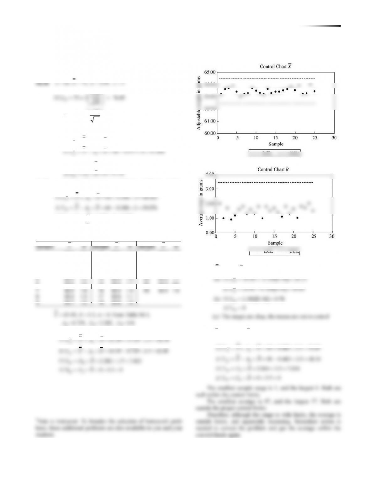
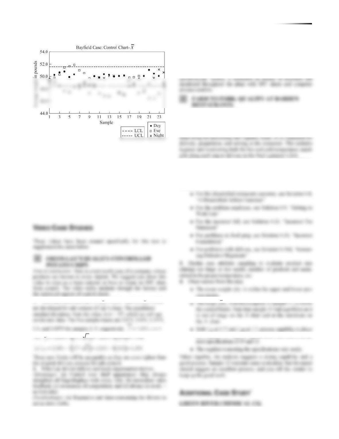
This is a very straightforward case. Running software to analyze
the data will generate the
UCLx
: 61.13
(Center line) Nominal: 49.78
LCLx
: 38.42
and the range chart as
UCLR : 41.62
(Center line) Nominal: 19.68
LCLR : 0.00
Next, students need to take the means and ranges for the five addi–
tional samples:
Date
Mean
Range
April
6
52
18
7
57
25
8
47
16
9
51.4
22
10
51.6
21
The mean and the ranges are all well within the control limits for
this week. There is, however, a noticeable change in the original
data at time 13, where the range suddenly dropped. It then goes
–chart asX
1.95
75 3 76.85
10
1.95
75 3 73.15
10
X
X
UCL
LCL
= + =
= − =
S6.37 n = 5. From Table S6.1, A2 = 0.577, D4 = 2.115, D3 = 0
2
2
(a) 50 0.577 4 52.308
50 0.577 4 47.692
X
X
UCL X A R
LCL X A R
= + = + =
= − = − =
4
3
(b) 2.115 4 8.456
0 4 0
R
R
UCL D R
LCL D R
= = =
= = =
S6.38 n = 10. From Table S6.1, A2 = 0.308, D4 = 1.777, D3 = 0.233
2
2
4
3
60 0.308 3 60.924
60 0.308 3 59.076
1.777 3 5.331
0.223 3 0.669
X
X
R
R
UCL X A R
LCL X A R
UCL D R
LCL D R
= + = + =
= − = − =
= = =
= = =
S6.39
Sample
X
R
Sample
X
R
Sample
X
R
1
63.5
2.0
10
63.5
1.3
19
63.8
1.3
2
63.6
1.0
11
63.3
1.8
20
63.5
1.6
3
63.7
1.7
12
63.2
1.0
21
63.9
1.0
4
63.9
0.9
13
63.6
1.8
22
63.2
1.8
5
63.4
1.2
14
63.3
1.5
23
63.3
1.7
6
63.0
1.6
15
63.4
1.7
24
64.0
2.0
7
63.2
1.8
16
63.4
1.4
25
63.4
1.5
8
63.3
1.3
17
63.5
1.1
9
63.7
1.6
18
63.6
1.8
= = =
= = =
2 4 3
63.49, 1.5, 4. From Table S6.1,
0.729, 2.282, 0.0.
X R n
A D D
2
2
4
3
63.49 0.729 1.5 64.58
63.49 0.729 1.5 62.40
2.282 1.5 3.423
0 1.5 0
X
X
R
R
UCL X A R
LCL X A R
UCL D R
LCR D R
= + = + =
= − = − =
= = =
= = =
S6.40
= = = = =
24
19.90, 0.34, 4, 0.729, 2.282X R n A D
()
()
= + =
= − =
(a) 19.90 0.729 0.34 20.15
19.90 0.729 0.34 19.65
X
X
UCL
LCL
()
==
=
(b) 2.282 0.34 0.78
0
R
R
UCL
LCL
S6.41
Desired Desired
3.5, 50, 6R X n= = =
= + = + =
= − = − =
= = =
= = =
2
2
3
4
50 0.483 3.5 51.69
50 0.483 3.5 48.31
2.004 3.5 7.014
0 3.5 0
X
X
R
R
UCL X A R
LCL X A R
UCL D R
LCL D R
The smallest sample range is 1, and the largest 6. Both are
well within the control limits.
The smallest average is 47, and the largest 57. Both are
outside the proper control limits.
Therefore, although the range is with limits, the average is
outside limits, and apparently increasing. Immediate action is
needed to correct the problem and get the average within the
con-trol limits again.
*Note to instructor: To broaden the selection of homework prob-
lems, these additional problems are also available to you and your
students.
90 SUPPLEMENT 6 ST A T I S T I C A L PR O C E S S CO N T R O L
S6.42 0.51
_ _ _ _ _ _ _ _ _ _ _ _ _ _ _ _ _ 0.505 drill bit (largest)
_ _ _ _ _ _ _ _ _ _ _ _ _ _ _ _ _ 0.495 drill bit (smallest)
0.49
0.505 – 0.49 = 0.015, 0.015/0.00017 = 88 holes within
standard
0.495 – 0.49 = 0.005, 0.005/0.00017 = 29 holes within
standard
Any one drill bit should produce at least 29 holes that meet
S6.45
Number
Number
Number
Day
Defective
Day
Defective
Day
Defective
1
6
8
3
15
4
2
5
9
6
16
5
3
6
10
3
17
6
4
4
11
7
18
5
5
3
12
5
19
4
6
4
13
4
20
3
SUPPLEMENT 6 ST A T I S T I C A L PR O C ES S CO N T R O L 91
19
21
0.105
Y
20
26
0.13
Y
21
28
0.14
Y
22
22
0.11
Y
23
17
0.085
Y
24
14
0.07
Y
25
12
0.06
Y
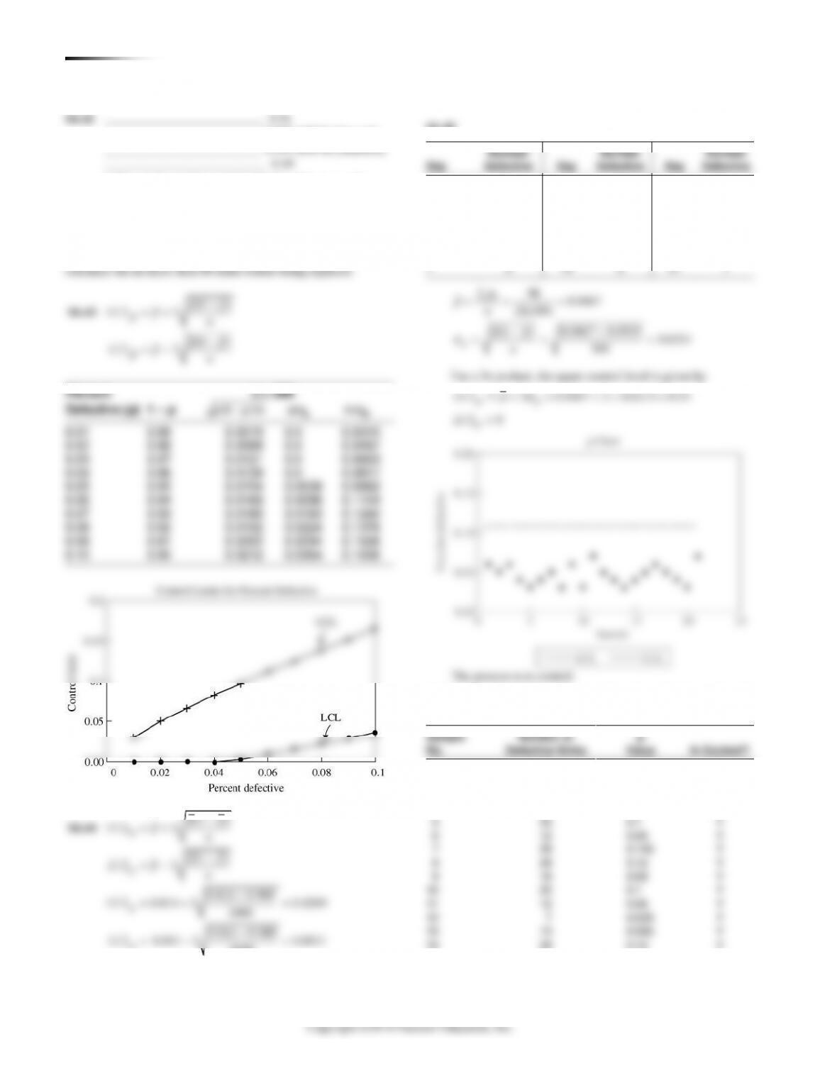
p-bar = 0.0924
Std. Deviation of p = 0.020477
UCLp = 0.154
LCLp = 0.031
The process is not in control as sample 16 exceeds the UCL.
When sample 16 is removed and the control limits recalculated,
the process is in control, based on the data. This points out the
importance of statistical sampling in process control.
S6.47
Total number of incidents/Total number of residents
156 /10,000 0.0156
(1 ) [(0.0156)(1 0.0156)]/1,000 0.0039
1,000
p
p
pp
=
==
−
= = − =
S6.49
Time
Box 1
Box 2
Box 3
Box 4
Average
9 AM
9.8
10.4
9.9
10.3
10.1
10 AM
10.1
10.2
9.9
9.8
10.0
11 AM
9.9
10.5
10.3
10.1
10.2
12 PM
9.7
9.8
10.3
10.2
10.0
1 PM
9.7
10.1
9.9
9.9
9.9
Average=
10.04
Std. Dev. =
0.11
10.1 10 10 9.9
0.3 and 0.3
(3)(0.11) (3)(0.11)
−−
==
As 0.3 is less than 1, the process will not produce within the
specified tolerance.
S6.50 Machine 1 produces “off–center” with a smaller standard
deviation than Machine 2. Machine 1 has index of 0.83, and
Machine 2 has an index of 1.0. Thus, Machine 1 is not capable.
Machine 2 is capable.
92 SUPPLEMENT 6 ST A T I S T I C A L PR O C E S S CO N T R O L
1. The first thing that must be done is to develop quality control
limits for the sample means. This can be done as follows. Because
the process appears to be unstable, we can use the desired mean as
a 99.73% confidence interval Z = 3:
3 50 3 0.489 50 1.47 51.47
3 50 1.47 48.53
Xx
Xx
UCL X
LCL X
= + = + = + =
= − = − =
Now that we have appropriate control limits, these must be
applied to the samples taken on the individual shifts:
Day Shift*
Time
Ave
Low
High
Ave
Low
High
Ave
Low
High
6:00
49.6
48.7
50.7
48.6
47.4
52.0
48.4
45.0
49.0
7:00
50.2
49.1
51.2
50.0
49.2
52.2
48.8
44.8
49.7
8:00
50.6
49.6
51.4
49.8
49.0
52.4
49.6
48.0
51.8
9:00
50.8
50.2
51.8
50.3
49.4
51.7
50.0
48.1
52.7
Evening Shift
Time
Ave
Low
High
Ave
Low
High
Ave
Low
High
2:00
49.0
46.0
50.6
49.7
48.6
51.0
49.8
48.4
51.0
3:00
49.8
48.2
50.8
48.4
47.2
51.7
49.8
48.8
50.8
4:00
50.3
49.2
52.7
47.2
45.3
50.9
50.0
49.1
50.6
5:00
51.4
50.0
55.3
46.8
44.1
49.0
47.8
45.2
51.2
6:00
51.6
49.2
54.7
46.8
41.0
51.2
46.4
44.0
49.7
7:00
51.8
50.0
55.6
50.0
46.2
51.7
46.5
44.4
50.0
8:00
51.0
48.6
53.2
47.4
44.0
48.7
47.2
46.6
48.9
Night Shift
Time
Ave
Low
High
Ave
Low
High
Ave
Low
High
10:00
49.2
46.1
50.7
47.2
46.6
50.2
49.2
48.1
50.7
11:00
49.0
46.3
50.8
48.6
47.0
50.0
48.4
47.0
50.8
3:00
48.2
45.2
49.0
50.0
49.2
50.0
49.6
49.0
50.6
4:00
48.0
45.5
49.1
47.2
46.3
50.5
51.0
50.5
51.5
5:00
48.4
47.1
49.6
47.0
44.1
49.7
50.5
50.0
51.9
* Boldfaced type indicates a sample outside the quality control limits.
(a) Day shift (6:00 A.M.–2:00 P.M.):
Number of means within control limits 23 96%
Total number of means 24
=→
(b) Evening shift (2:00 P.M.–10:00 P.M.):
Number of means within control limits 12 50%
Total number of means 24
=→
(c) Night shift (10:00 P.M.–6:00 A.M.):
Total number of means 24
As is now evident, none of the shifts meet the control specifi-
cations. Bag weight monitoring needs improvement on all shifts.
The problem is much more acute on the evening and night shifts
weight” is much greater than the number indicating excess weight.
With regard to the range, 99.73% of the individual bag
weights should lie within 3 of the mean. This would represent a
range of 6, or 7.2. Only one of the ranges defined by the differ–
ence between the highest and lowest bag weights in each sample
exceeds this range. Alternatively: D4 × Sample range = UCLR and
D2 × Sample range = LCLR. This is dangerous if the process is out
of control, but the mean range for the first shift is 3.14 (the lowest
of any shift) and D4 × 3.14 = 6.28 and D3 × 3.14 = 0. A range of
0 to 6.28 compares favorably with 7.2, with only two values
exceeding the range limit. It would appear, then, that the problem
is not due to abnormal deviations between the highest and lowest
bag weights, but rather to poor adjustments of the bag weight-
of 6, or 7.2. Only one of the ranges defined by the differ-ence
between the highest and lowest bag weights in each sample ex-
ceeds this range. Alternatively: D4 × Sample range = UCLR and
D2 × Sample range = LCLR. This is dangerous if the process is out
of control, but the mean range for the first shift is 3.14 (the lowest
of any shift) and D4 × 3.14 = 6.28 and D3 × 3.14 = 0. A range of
0 to 6.28 compares favorably with 7.2, with only two values ex-
ceeding the range limit. It would appear, then, that the problem is
not due to abnormal deviations between the highest and lowest
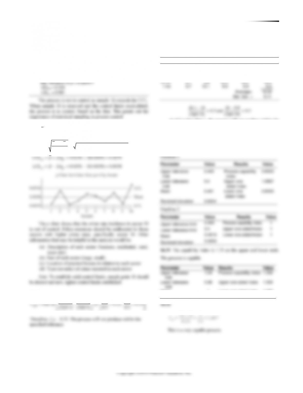
2. The proper procedure is to establish mean and range charts
to guide the bag packers. The foreman would then be alerted
when sample weights deviate from mean and range control limits.
The immediate problem, however, must be corrected by additional
94 SUPPLEMENT 6 ST A T I S T I C A L PR O C E S S CO N T R O L
This is a very straightforward case. Running software to analyze
the data will generate the
UCLx
: 61.13
(Center line) Nominal: 49.78
LCLx
: 38.42
and the range chart as
UCLR : 41.62
(Center line) Nominal: 19.68
LCLR : 0.00
Next, students need to take the means and ranges for the five addi–
tional samples:
Date
Mean
Range
April
6
52
18
7
57
25
8
47
16
9
51.4
22
10
51.6
21
The mean and the ranges are all well within the control limits for
this week. There is, however, a noticeable change in the original
data at time 13, where the range suddenly dropped. It then goes
–chart asX