6
S U P P L E M E N T
Statistical Process Control
1. Shewhart’s two types of variation, common and special caus-
es, are also called natural and assignable variation.
2. A process is said to be operating in statistical control when
the only source of variation is natural or common causes.
3. The x-bar chart indicates whether changes have occurred in
the central tendency of a process; the R-chart indicates whether a
gain or a loss in uniformity has occurred.
4. A process can be out of control because of assignable varia-
tion, which can be traced to specific causes. Examples include
such factors as:
5. The 5 steps are:
1. Collect 20 to 25 samples, often of n = 4 or 5 each;
compute the mean and range of each sample.
acceptable limits.
4. Investigate points or patterns that indicate the process is
out of control. Try to assign causes for the variation,
address the causes, and then resume the process.
5. Collect additional samples and, if necessary, revalidate the
control limits using the new data.
6. Text list includes machine wear, misadjusted equipment,
fatigued or untrained workers, new batches of raw materials, etc.
Others might be bad measuring device, workplace lighting, other
7. Two sigma covers only 95.5% of all natural variation; even in
the absence of assignable cause, points will fall outside the control
limits 4.5% of the time.
we are doing something “too well,” then the process has changed
from the norm. We want to find out what we are doing “too well” so
10. Control charts are designed for specific sample sizes because
the sample standard deviation or range is dependent on the sample
size. The control charts presented here should not be used if the
11. Cpk, the process capability index, is one way to express
process capability. It measures the proportion of natural variation
(3) between the center of the process and the nearest specifica-
are combined with risk levels to determine an acceptance sam-
14. A run test is used to help spot abnormalities in a control
chart process. It is used if points are not individually out of con-
16. An OC curve is a graph showing the probability of accepting
a lot given a certain quality (percentage of defective).
17. The purpose of acceptance sampling is to determine a course
of action (accept or reject) regarding the disposition of a lot with-
out inspecting each item in a lot. Acceptance sampling does not
18. The two risks when acceptance sampling is used are type I
error: rejecting a good lot; type II error: accepting a bad lot.
“capable” process—produces small percentages of unacceptable
items. The capability formula is built around an assumption of
exactly one, those parts that are more than three sigma from center
82 SUPPLEMENT 6 ST A T I S T I C A L PR O C E S S CO N T R O L
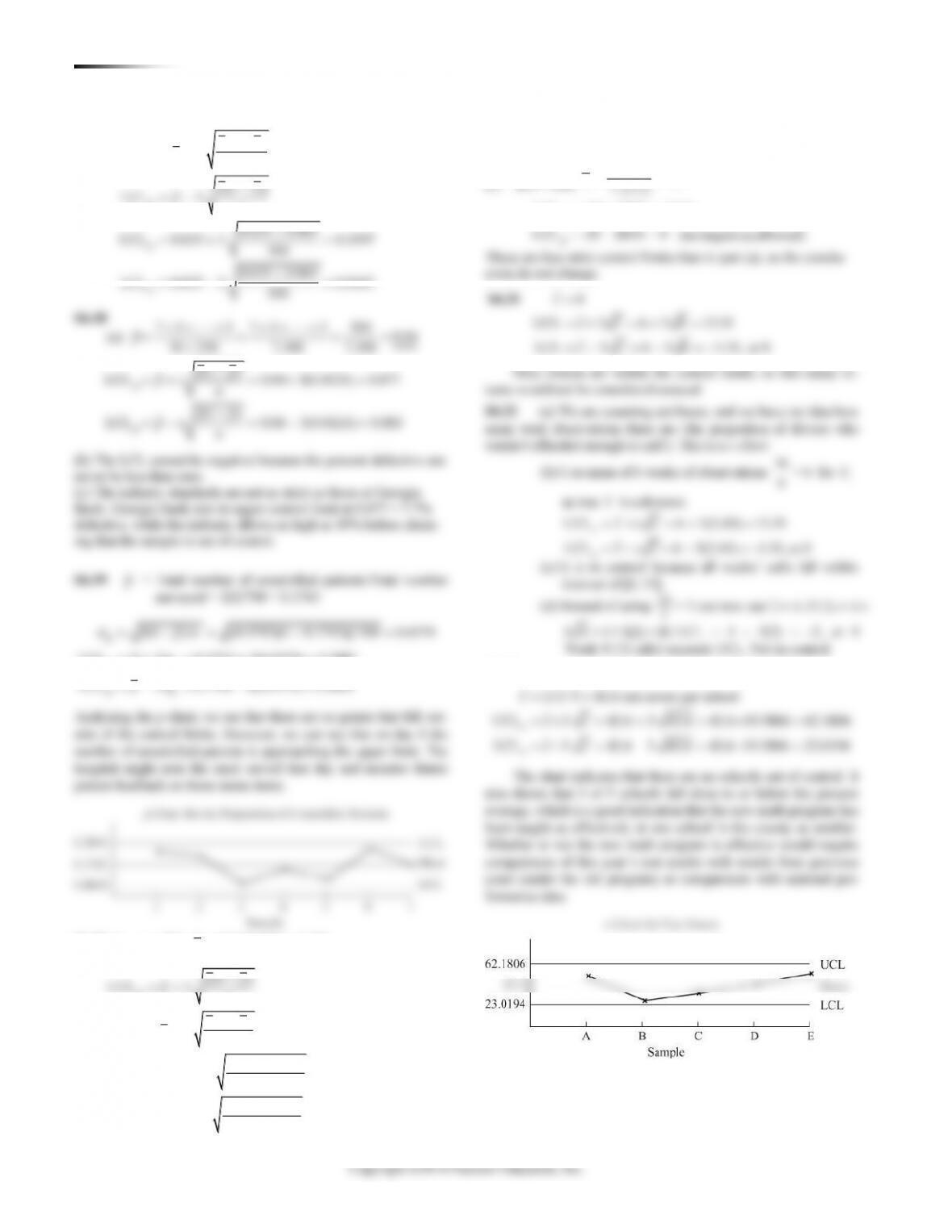
1. Has the process been in control?
No, three points are out of control. One is above the UCL, and
two are below the LCL.
2. If we use a two-sigma control chart, what are the UCL and
LCL? Is the process more out of control?
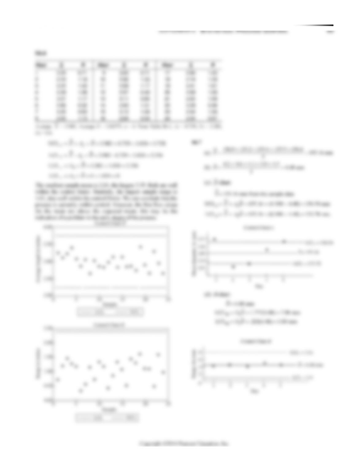
The control limits are tighter. UCL = 16.667 and LCL =
15.333. Now five points are out of control.
3. What happens if the Z-value increases?
Now the control limits are wider at Z = 4, only one point is
out of control.
4. What happens if variance in package weight is reduced?
The control limits become tighter. For example, if
population standard deviation drops from 1 to 0.5, UCL = 16.33
1. Has the process been in control?
Samples 3 and 19 were “too good,” and sample 16 was out of
control.
2. Suppose we use a 95% p-chart. What are the upper and lower
control limits? Has the process gotten more out of control?
.074 and .0008. It is the same process but sample 13 is also
3. Suppose that the sample size used was actually 120 instead of
the 100 that it was supposed to be. How does this affect the chart?
The overall percentage of defects drops and, in addition,
the UCL and LCL get closer to the center line and each other.
4. What happens to the chart as we reduce the Z-value?
6. What happens to the actual alpha and beta as the critical val-
ue, c, is increased?
Alpha decreases and beta increases.
S6.1
0.1 0.1 0.0167
6
36
xn
= = = =
= 14 oz.
UCL 14 3 14 3(0.0167) 14 0.05 14.05 oz.
LCL 14 3 14 3(0.0167) 13.95 oz.
x
x
= + = + = + =
= − = − =
S6.2(a)
5, 50, 1.72, 3
X
nz
= = = =
1.72
50 3 47.69
5
X
LCL
= − =
( )
( )
(b) = 2
1.72
U CL 50 2 50 2 .77 51.54.
5
LCL 50 50 .77 48.46
5
Z
x
x
= + = + =
= = =
– 2 – 2
The control limits are tighter, but the confidence level has dropped.
S6.3 The relevant constants are:
2 4 3
= 0.419 =1.924 = 0.076A D D
84 SUPPLEMENT 6 ST A T I S T I C A L PR O C E S S CO N T R O L
(e) If the desired nominal line is 155 mm, then:
U CL 155 (.308 4.48) 155 1.38 156.38
X
= + = + =
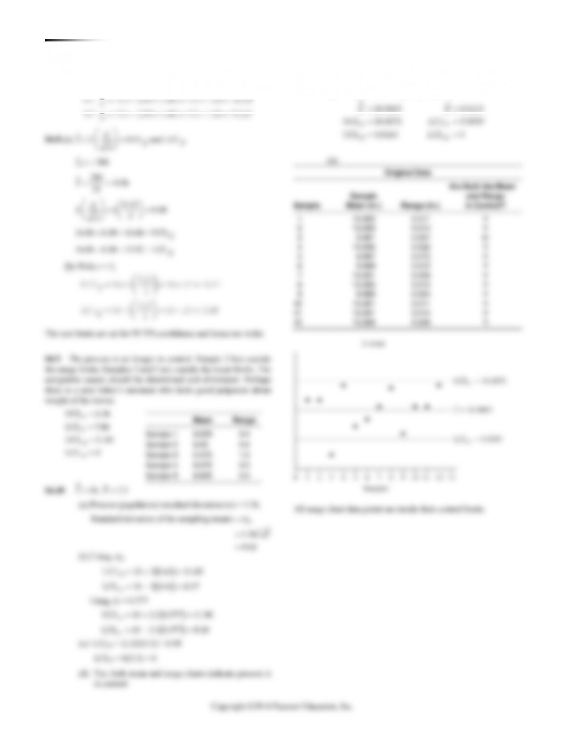
S6.11
= = =
==
2 4 3
(a) .577, 2.115, 0
10.0005 0.0115
A D D
XR
2 4 3
0.577, 2.115, 0 A D D= = =
10.0023 0.0119
UCL 10.0091 LCL 9.9954
UCL 0.0252 LCL 0
xx
RR
XR==
==
==
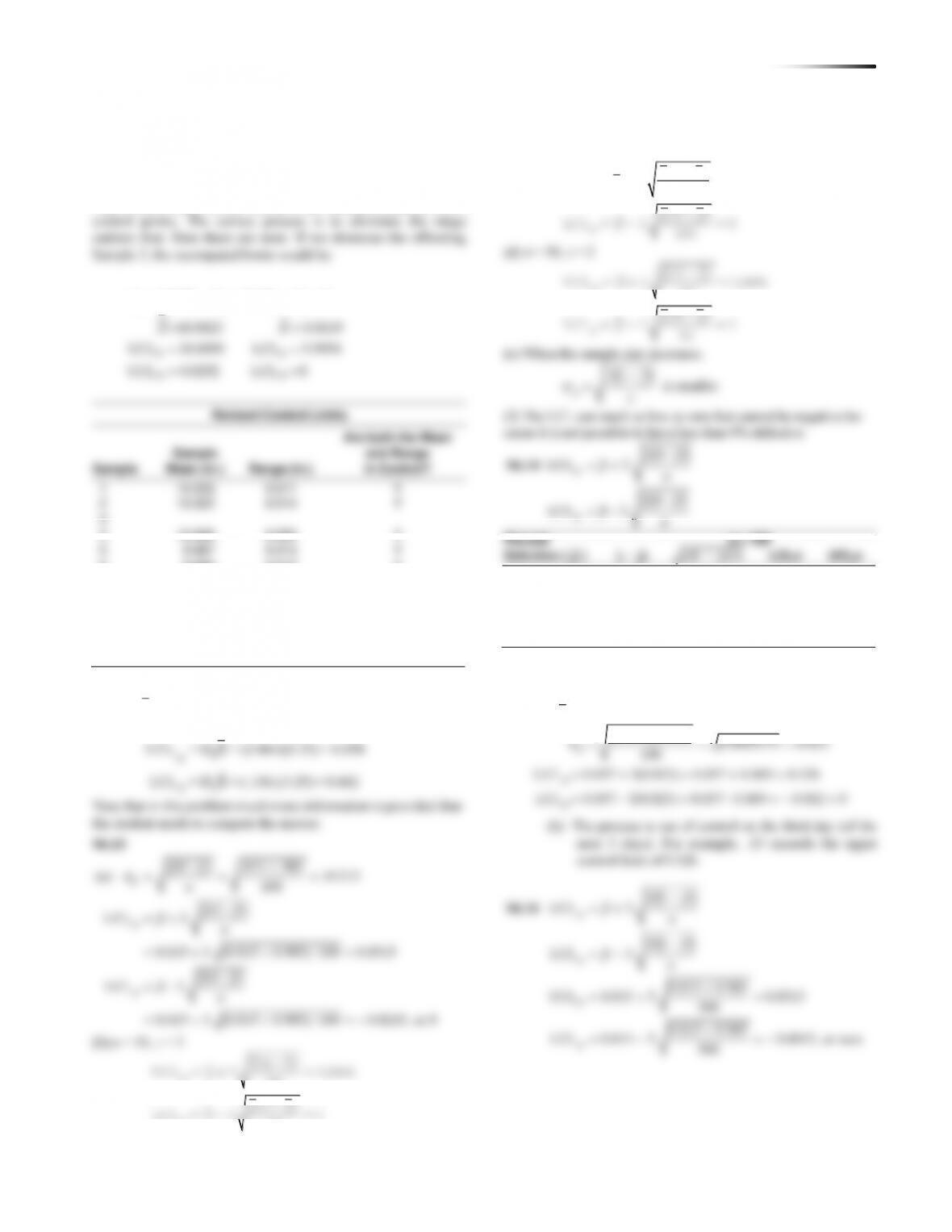
Revised Control Limits
Are both the Mean
Sample
and Range
Sample
Mean (in.)
Range (in.)
in Control?
1
10.002
0.011
Y
2
10.002
0.014
Y
3
4
10.006
0.022
Y
5
9.997
0.013
Y
6
9.999
0.012
Y
7
10.001
0.008
Y
8
10.005
0.013
Y
9
9.995
0.004
Y
10
10.001
0.011
Y
11
10.001
0.014
Y
12
10.006
0.009
Y
These limits reflect a process that is now in control.
S6.12
R= 3.25
mph, Z = 3,with n = 8, from Table S6.1, D4 =
1.864, D3 = .136
S6.13
−
= = =
−
=+
= + =
−
=−
= − = −
(1 ) .015 .985
(a) .01215
100
(1 )
UCL 3
0.015 3 (0.015 0.985) / 100 0.0515
(1 )
LCL 3
0.015 3 (0.015 0.985) / 100 0.0215, or 0
p
p
p
pp
n
pp
pn
pp
pn
(b) n = 50, z = 3
(1 )
U CL 3 0.0666
p
pp
p
−
= + =
U CL 2 0.0494
50
(1 )
LCL 2 0
50
p
p
p
pp
p
= + =
−
= − =
(e) When the sample size increases,
()
1
p
pp
n
−
=
is smaller.
(f) The LCL can reach as low as zero but cannot be negative be-
cause it is not possible to have less than 0% defective.
( )
( )
1
UCL 3
1
LCL 3
p
p
pp
pn
pp
pn
−
=+
−
=−
S6.14
Percent
n = 100
Defective (
p
)
−1p
−(1 )ppn
LCLP
UCLP
0.02
0.98
0.014
0.0
0.062
0.04
0.96
0.020
0.0
0.099
0.06
0.94
0.024
0.0
0.132
0.08
0.92
0.027
0.0
0.161
0.10
0.90
0.030
0.01
0.190
S6.15 (a) The total number defective is 57.
57 / 1,000 0.057
(0.057)(0.943) 0.0005375 0.023
100
UCL 0.057 3(0.023) 0.057 0.069 0.126
p
p
p
==
= = =
=+ =+=
next 3 days). For example, .13 exceeds the upper
control limit of 0.126.
()
()
1
UCL 3
1
LCL 3
0.015 0.985
UCL 0.015 3 0.0313
500
0.015 0.985
LCL 0.015 3 0.0013, or zero
500
p
p
p
p
pp
pn
pp
pn
S6.16 −
=+
−
=−
= + =
= − = −
4
UCL = D R = (1.864)(3.25) = 6.058
LCL = D R = (.136) (3.25) = 0.442
R
86 SUPPLEMENT 6 ST A T I S T I C A L PR O C E S S CO N T R O L
()
()
1
UCL 3
1
LCL 3
0.035 0.965
UCL 0.035 3 0.0597
500
0.035 0.965
LCL 0.035 3 0.0103
500
p
p
p
p
pp
pn
pp
pn
S6.17 −
=+
−
=−
= + =
= − =
S6.18
S6.19
p
= Total number of unsatisfied patients/Total number
(b) The highest percent defective is .04; therefore, the process is
in control.
(c) If n = 100,
50 .05
10(100)
p==
UCL = .05 + .0654 = .1154
LCL = .05 – .0654 = 0 (no negatives allowed)
p
p
These are less strict control limits than in part (a), so the conclu-
sions do not change.
6
UCL 3 6 3 6 13.35
LCL 3 6 3 6 1.35, or 0
c
cc
cc
=
= + = + =
= − = − = −
S6.21
Nine returns are within the control limits; so this many re–
(c) It is in control because all weeks’ calls fall within
interval of [0, 13].
+ + + + + +
= = = =
−
= + = + =
. . . . . .
7 5 3 7 5 3 300
(a) 0.04
30 250 7,500 7,500
(1 )
UCL 0.04 3(0.0124) 0.077
p
p
pp
pz n
SUPPLEMENT 6 ST A T I S T I C A L PR O C E S S CO N T R O L 87
S6.24
(a) 73/ 5 14.6 nonconformities per day
UCL 3 14.6 3 14.6 14.6 11.4630 26.063
LCL 3 14.6 3 14.6 14.6 11.4630 3.137
c
c
c
cc
cc
==
= + = + = + =
= − = − = − =
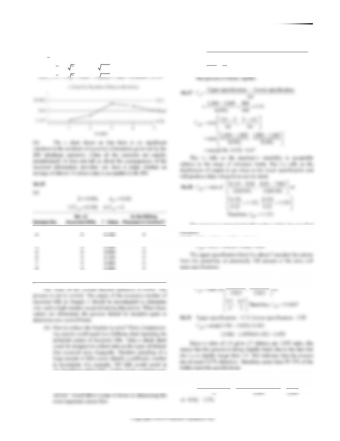
(b) The c chart shows us that there is no significant
variation in the incidents of incorrect information given out by the
IRS telephone operators. (Thus all the operators are equally
misinformed!) It does not tell us about the consequences of the
incorrect information provided, nor does it judge whether an
average of almost 15 errors a day is acceptable to the IRS.
S6.25
(a)
0.094, 0.041
UCL 0.218 LCL 0
p
pp
p
==
==
No. of
Is the Billing
Sample No.
Incorrect Bills
p
Value
Process in Control?
1
6
0.120
Y
2
5
0.100
Y
3
11
0.220
N
4
4
0.080
Y
5
0
0.000
Y
6
5
0.100
Y
7
3
0.060
Y
4
4
0.080
Y
5
0
0.000
Y
6
5
0.100
Y
7
3
0.060
Y
8
4
0.080
Y
9
7
0.140
Y
10
2
0.040
Y
The value of the overall fraction defective is 0.094. The
process is not in control. The causes of the excessive number of
incorrect bills in Sample 3 should be investigated to determine
25–30 defective bills (300 × 9.4%). Each would be stud-
ied and the types of errors noted. Then a Pareto chart
could be constructed showing which types of errors oc-
curred most frequently. This identification of the “criti-
=
= = =
Difference between upper and lower specifications
6
.6 .6 1.0
6(.1) .6
p
CS6.26
This process is barely capable.
Upper specification Lower specification
6
2,400 1,600 800 1.33
6(100) 600
p
C
−
=
−
= = =
S6.27
min ,
33
2,400 1,800 1,800 1,600
min ,
3(100) 3(100)
min [2.00, 0.67] = 0.67
pk
USL x x LSL
C
−−
=
−−
=
=
The Cp tells us the machine’s variability is acceptable
relative to the range of tolerance limits. But Cpk tells us the
distribution of output is too close to the lower specification and
will produce chips whose lives are too short.
−−
=
==
=
8.135 8.00 8.00 7.865
min of , or
(3)(0.04) (3)(0.04)
0.135 0.135
1.125, 1.125
0.12 0.12
Therefore, 1.125.
pk
pk
C
C
S6.28
The process is centered and will produce within the specified
S6.29 LSL = 2.9 mm, USL = 3.1 mm
S6.30
−−
=
=
16.5 16 16 15.5
min of , or
(3)(1) (3)(1)
0.5 0.5
, Therefore, 0.1667
pk
pk
C
C
bottles meet the specifications.
S6.32
( )( )( – ) (.03)(.79)(1,000 – 80) 21.80
AOQ .022
1,000 1,000
da
P P N n
N
= = =
82 SUPPLEMENT 6 ST A T I S T I C A L PR O C E S S CO N T R O L
1. Has the process been in control?
No, three points are out of control. One is above the UCL, and
two are below the LCL.
2. If we use a two-sigma control chart, what are the UCL and
LCL? Is the process more out of control?
The control limits are tighter. UCL = 16.667 and LCL =
15.333. Now five points are out of control.
3. What happens if the Z-value increases?
Now the control limits are wider at Z = 4, only one point is
out of control.
4. What happens if variance in package weight is reduced?
The control limits become tighter. For example, if
population standard deviation drops from 1 to 0.5, UCL = 16.33
1. Has the process been in control?
Samples 3 and 19 were “too good,” and sample 16 was out of
control.
2. Suppose we use a 95% p-chart. What are the upper and lower
control limits? Has the process gotten more out of control?
.074 and .0008. It is the same process but sample 13 is also
3. Suppose that the sample size used was actually 120 instead of
the 100 that it was supposed to be. How does this affect the chart?
The overall percentage of defects drops and, in addition,
the UCL and LCL get closer to the center line and each other.
4. What happens to the chart as we reduce the Z-value?
6. What happens to the actual alpha and beta as the critical val-
ue, c, is increased?
Alpha decreases and beta increases.
S6.1
0.1 0.1 0.0167
6
36
xn
= = = =
= 14 oz.
UCL 14 3 14 3(0.0167) 14 0.05 14.05 oz.
LCL 14 3 14 3(0.0167) 13.95 oz.
x
x
= + = + = + =
= − = − =
S6.2(a)
5, 50, 1.72, 3
X
nz
= = = =
1.72
50 3 47.69
5
X
LCL
= − =
( )
( )
(b) = 2
1.72
U CL 50 2 50 2 .77 51.54.
5
LCL 50 50 .77 48.46
5
Z
x
x
= + = + =
= = =
– 2 – 2
The control limits are tighter, but the confidence level has dropped.
S6.3 The relevant constants are:
2 4 3
= 0.419 =1.924 = 0.076A D D
84 SUPPLEMENT 6 ST A T I S T I C A L PR O C E S S CO N T R O L
(e) If the desired nominal line is 155 mm, then:
U CL 155 (.308 4.48) 155 1.38 156.38
X
= + = + =
S6.11
= = =
==
2 4 3
(a) .577, 2.115, 0
10.0005 0.0115
A D D
XR
2 4 3
0.577, 2.115, 0 A D D= = =
10.0023 0.0119
UCL 10.0091 LCL 9.9954
UCL 0.0252 LCL 0
xx
RR
XR==
==
==
Revised Control Limits
Are both the Mean
Sample
and Range
Sample
Mean (in.)
Range (in.)
in Control?
1
10.002
0.011
Y
2
10.002
0.014
Y
3
4
10.006
0.022
Y
5
9.997
0.013
Y
6
9.999
0.012
Y
7
10.001
0.008
Y
8
10.005
0.013
Y
9
9.995
0.004
Y
10
10.001
0.011
Y
11
10.001
0.014
Y
12
10.006
0.009
Y
These limits reflect a process that is now in control.
S6.12
R= 3.25
mph, Z = 3,with n = 8, from Table S6.1, D4 =
1.864, D3 = .136
S6.13
−
= = =
−
=+
= + =
−
=−
= − = −
(1 ) .015 .985
(a) .01215
100
(1 )
UCL 3
0.015 3 (0.015 0.985) / 100 0.0515
(1 )
LCL 3
0.015 3 (0.015 0.985) / 100 0.0215, or 0
p
p
p
pp
n
pp
pn
pp
pn
(b) n = 50, z = 3
(1 )
U CL 3 0.0666
p
pp
p
−
= + =
U CL 2 0.0494
50
(1 )
LCL 2 0
50
p
p
p
pp
p
= + =
−
= − =
(e) When the sample size increases,
()
1
p
pp
n
−
=
is smaller.
(f) The LCL can reach as low as zero but cannot be negative be-
cause it is not possible to have less than 0% defective.
( )
( )
1
UCL 3
1
LCL 3
p
p
pp
pn
pp
pn
−
=+
−
=−
S6.14
Percent
n = 100
Defective (
p
)
−1p
−(1 )ppn
LCLP
UCLP
0.02
0.98
0.014
0.0
0.062
0.04
0.96
0.020
0.0
0.099
0.06
0.94
0.024
0.0
0.132
0.08
0.92
0.027
0.0
0.161
0.10
0.90
0.030
0.01
0.190
S6.15 (a) The total number defective is 57.
57 / 1,000 0.057
(0.057)(0.943) 0.0005375 0.023
100
UCL 0.057 3(0.023) 0.057 0.069 0.126
p
p
p
==
= = =
=+ =+=
next 3 days). For example, .13 exceeds the upper
control limit of 0.126.
()
()
1
UCL 3
1
LCL 3
0.015 0.985
UCL 0.015 3 0.0313
500
0.015 0.985
LCL 0.015 3 0.0013, or zero
500
p
p
p
p
pp
pn
pp
pn
S6.16 −
=+
−
=−
= + =
= − = −
4
UCL = D R = (1.864)(3.25) = 6.058
LCL = D R = (.136) (3.25) = 0.442
R
86 SUPPLEMENT 6 ST A T I S T I C A L PR O C E S S CO N T R O L
()
()
1
UCL 3
1
LCL 3
0.035 0.965
UCL 0.035 3 0.0597
500
0.035 0.965
LCL 0.035 3 0.0103
500
p
p
p
p
pp
pn
pp
pn
S6.17 −
=+
−
=−
= + =
= − =
S6.18
S6.19
p
= Total number of unsatisfied patients/Total number
(b) The highest percent defective is .04; therefore, the process is
in control.
(c) If n = 100,
50 .05
10(100)
p==
UCL = .05 + .0654 = .1154
LCL = .05 – .0654 = 0 (no negatives allowed)
p
p
These are less strict control limits than in part (a), so the conclu-
sions do not change.
6
UCL 3 6 3 6 13.35
LCL 3 6 3 6 1.35, or 0
c
cc
cc
=
= + = + =
= − = − = −
S6.21
Nine returns are within the control limits; so this many re–
(c) It is in control because all weeks’ calls fall within
interval of [0, 13].
+ + + + + +
= = = =
−
= + = + =
. . . . . .
7 5 3 7 5 3 300
(a) 0.04
30 250 7,500 7,500
(1 )
UCL 0.04 3(0.0124) 0.077
p
p
pp
pz n
SUPPLEMENT 6 ST A T I S T I C A L PR O C E S S CO N T R O L 87
S6.24
(a) 73/ 5 14.6 nonconformities per day
UCL 3 14.6 3 14.6 14.6 11.4630 26.063
LCL 3 14.6 3 14.6 14.6 11.4630 3.137
c
c
c
cc
cc
==
= + = + = + =
= − = − = − =
(b) The c chart shows us that there is no significant
variation in the incidents of incorrect information given out by the
IRS telephone operators. (Thus all the operators are equally
misinformed!) It does not tell us about the consequences of the
incorrect information provided, nor does it judge whether an
average of almost 15 errors a day is acceptable to the IRS.
S6.25
(a)
0.094, 0.041
UCL 0.218 LCL 0
p
pp
p
==
==
No. of
Is the Billing
Sample No.
Incorrect Bills
p
Value
Process in Control?
1
6
0.120
Y
2
5
0.100
Y
3
11
0.220
N
8
4
0.080
Y
9
7
0.140
Y
10
2
0.040
Y
The value of the overall fraction defective is 0.094. The
process is not in control. The causes of the excessive number of
incorrect bills in Sample 3 should be investigated to determine
25–30 defective bills (300 × 9.4%). Each would be stud-
ied and the types of errors noted. Then a Pareto chart
could be constructed showing which types of errors oc-
curred most frequently. This identification of the “criti-
=
= = =
Difference between upper and lower specifications
6
.6 .6 1.0
6(.1) .6
p
CS6.26
This process is barely capable.
Upper specification Lower specification
6
2,400 1,600 800 1.33
6(100) 600
p
C
−
=
−
= = =
S6.27
min ,
33
2,400 1,800 1,800 1,600
min ,
3(100) 3(100)
min [2.00, 0.67] = 0.67
pk
USL x x LSL
C
−−
=
−−
=
=
The Cp tells us the machine’s variability is acceptable
relative to the range of tolerance limits. But Cpk tells us the
distribution of output is too close to the lower specification and
will produce chips whose lives are too short.
−−
=
==
=
8.135 8.00 8.00 7.865
min of , or
(3)(0.04) (3)(0.04)
0.135 0.135
1.125, 1.125
0.12 0.12
Therefore, 1.125.
pk
pk
C
C
S6.28
The process is centered and will produce within the specified
S6.29 LSL = 2.9 mm, USL = 3.1 mm
S6.30
−−
=
=
16.5 16 16 15.5
min of , or
(3)(1) (3)(1)
0.5 0.5
, Therefore, 0.1667
pk
pk
C
C
bottles meet the specifications.
S6.32
( )( )( – ) (.03)(.79)(1,000 – 80) 21.80
AOQ .022
1,000 1,000
da
P P N n
N
= = =