42
70.90
49.84
43
79.10
51.4782
44
94.00
53.1165
1,671.46
AVERAGE
22.50
17.893
(MSE)
40
55.80
43.5357
12.2643
150.412
41
70.10
44.8951
25.20
635.288
42
70.90
44.8951
26.00
676.256
43
79.10
46.2544
32.8456
44
94.00
50.3325
43.6675
TOTALS
451.223
AVERAGE
10.2551
204.92
(MAD)
(a)
(b)
13.5936
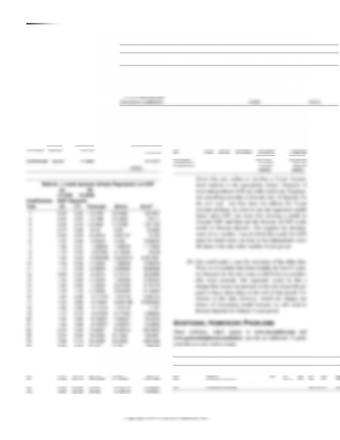
Coefficients:
GSP
Deposits
1
0.25
12.4482
154.957
2
0.24
12.4382
154.71
3
0.24
11.0788
122.740
4
8.38
70.226
5
0.25
5.65137
31.94
6
0.30
4.342
7
0.31
1.39545
1.08545
8
5.15354
26.56
9
0.24
0.203914
0.041581
10
0.26
1.58328
11
0.25
2.93264
12
0.33
5.73137
13
0.50
1.82328
14
0.95
2.27328
15
1.70
3.02328
16
2.30
4.11418
1.81418
17
2.80
2.75481
0.045186
0.002042
18
2.80
4.11418
1.31418
1.727
19
2.70
5.47354
2.77354
20
3.90
8.19227
4.29227
21
4.90
8.19227
3.29227
22
5.30
13.6297
8.32972
23
6.20
16.3484
10.1484
102.991
24
4.10
20.4265
16.3265
266.556
25
4.50
21.79
17.29
298.80
26
6.10
28.5827
22.4827
505.473
27
7.70
34.02
26.32
692.752
28
38.0983
27.9983
783.90
29
15.20
36.74
21.54
463.924
30
18.10
36.74
18.64
347.41
31
24.10
35.3795
11.2795
127.228
32
8.42018
33
3.72018
34
3.33918
35
31.10
38.0983
6.99827
36
6.39827
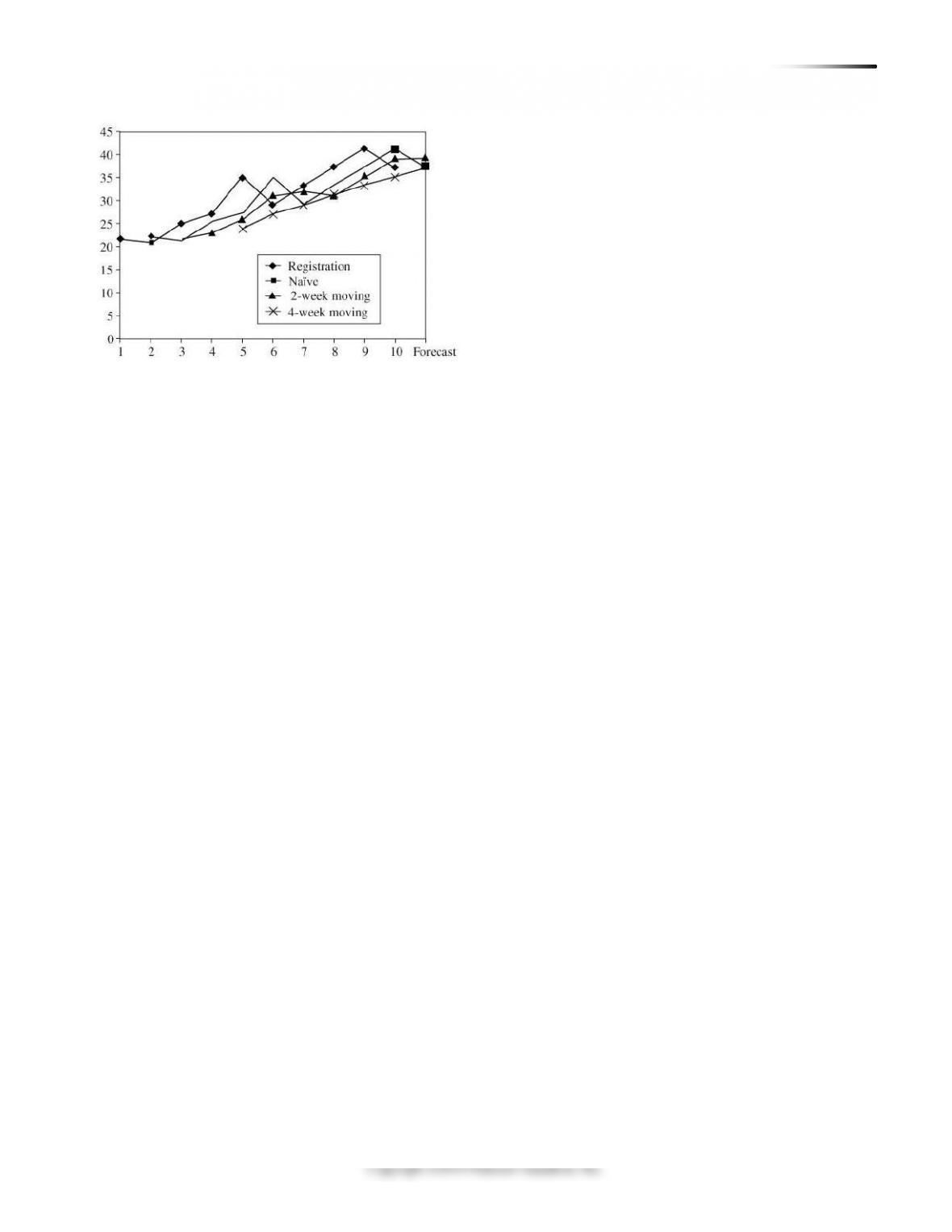
Week
1
2
3
4
5
6
Registration
22
21
25
27
35
29
(a)
Naïve
22
21
25
27
35
(b)
2-week moving
21.5
23
26
31
46 CHAPTER 4 FO R E C A S T I N G
39
49.10
44.9250
40
46.5633
41
41
70.10
48.2016
37
38.50
36.74
1.76
38
47.90
43.5357
4.36428
19.05
39
49.10
44.8951
4.20491
Method Used
13.59364 × GSP
MAD
10.255
MSE
204.919
Standard error using
Correlation coefficient
CHAPTER 4 FO R E C A ST I N G 47
Copyright ©2014 Pearson Education, Inc.
48 CHAPTER 4 FO R E C A S T I N G
4.51
Period
Demand
Exponentially Smoothed Forecast
1
7
5
2
9
5 + 0.2 × (7 – 5) = 5.4
3
5
5.4 + 0.2 × (9 – 5.4) = 6.12
4
9
6.12 + 0.2 × (5 – 6.12) = 5.90
3
5
5.4 + 0.2 × (9 – 5.4) = 6.12
4
9
6.12 + 0.2 × (5 – 6.12) = 5.90
5
13
5.90 + 0.2 × (9 – 5.90) = 6.52
6
8
6.52 + 0.2 × (13 – 6.52) = 7.82
7
Forecast
7.82 + 0.2 × (8 – 7.82) = 7.86
4.52
Actual
Forecast
|Error|
Error2
95
100
5
25
108
110
2
4
123
120
3
9
130
130
0
0
10
38
MAD = 10/4 = 2.5, MSE = 38/4 = 9.5
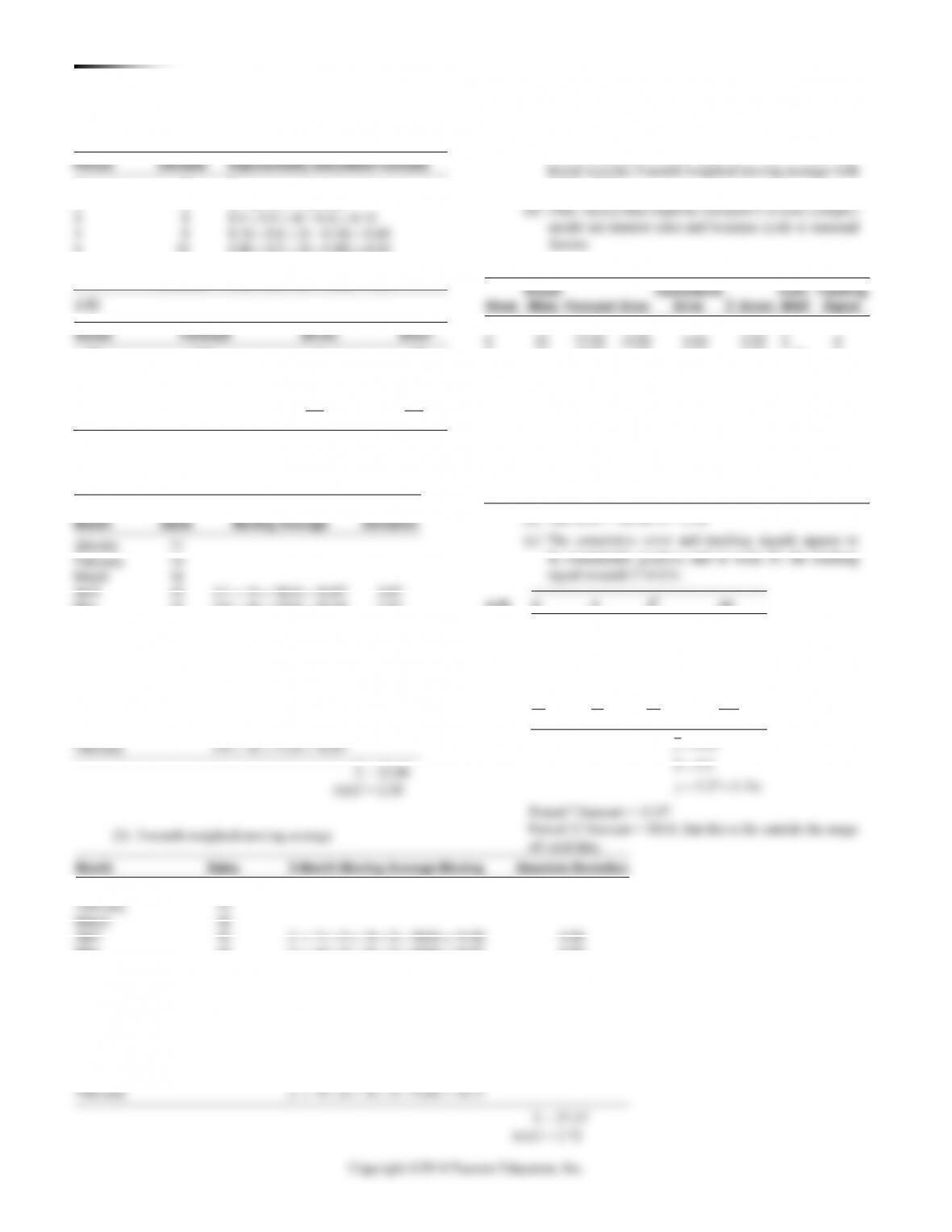
4.53 (a) 3-month moving average:
3-Month
Absolute
Month
Sales
Moving Average
Deviation
January
11
February
14
March
February
14
March
April
10
(11 + 14 + 16)/3 = 13.67
3.67
May
15
(14 + 16 + 10)/3 = 13.33
1.67
June
17
(16 + 10 + 15)/3 = 13.67
3.33
July
11
(10 + 15 + 17)/3 = 14.00
3.00
August
14
(15 + 17 + 11)/3 = 14.33
0.33
September
17
(17 + 11 + 14)/3 = 14.00
3.00
October
12
(11 + 14 + 17)/3 = 14.00
2.00
November
14
(14 + 17 + 12)/3 = 14.33
0.33
December
16
(17 + 12 + 14)/3 = 14.33
1.67
January
11
(12 + 14 + 16)/3 = 14.00
3.00
February
(14 + 16 + 11)/3 = 13.67
= 22.00
MAD = 2.20
(b) 3-month weighted moving average
(c) Based on a mean absolute deviation criterion, the
3-month moving average with MAD = 2.2 is to be pre-
ferred over the 3-month weighted moving average with
MAD = 2.72.
4.54 (a)
Actual
Cumulative
Cum.
Tracking
Week
Miles
Forecast
Error
Error
|Error|
MAD
Signal
1
17
17.00
0.00
–
0.00
0
2
21
17.00
+4.00
4.00
4.00
2
2
3
19
17.80
+1.20
5.20
5.20
1.73
3
4
23
18.04
+4.96
10.16
10.16
2.54
4
5
18
19.03
–1.03
9.13
11.19
2.24
4
6
16
18.83
–2.83
6.30
14.02
2.34
2.7
7
20
18.26
+1.74
8.04
15.76
2.25
3.6
8
18
18.61
–0.61
7.43
16.37
2.05
3.6
9
22
18.49
+3.51
10.94
19.88
2.21
5
10
20
19.19
+0.81
11.75
20.69
2.07
5.7
11
15
19.35
–4.35
7.40
25.04
2.28
3.2
12
22
18.48
+3.52
10.92
28.56
2.38
4.6
(b) The MAD = 28.56/12 = 2.38
(c) The cumulative error and tracking signals appear to
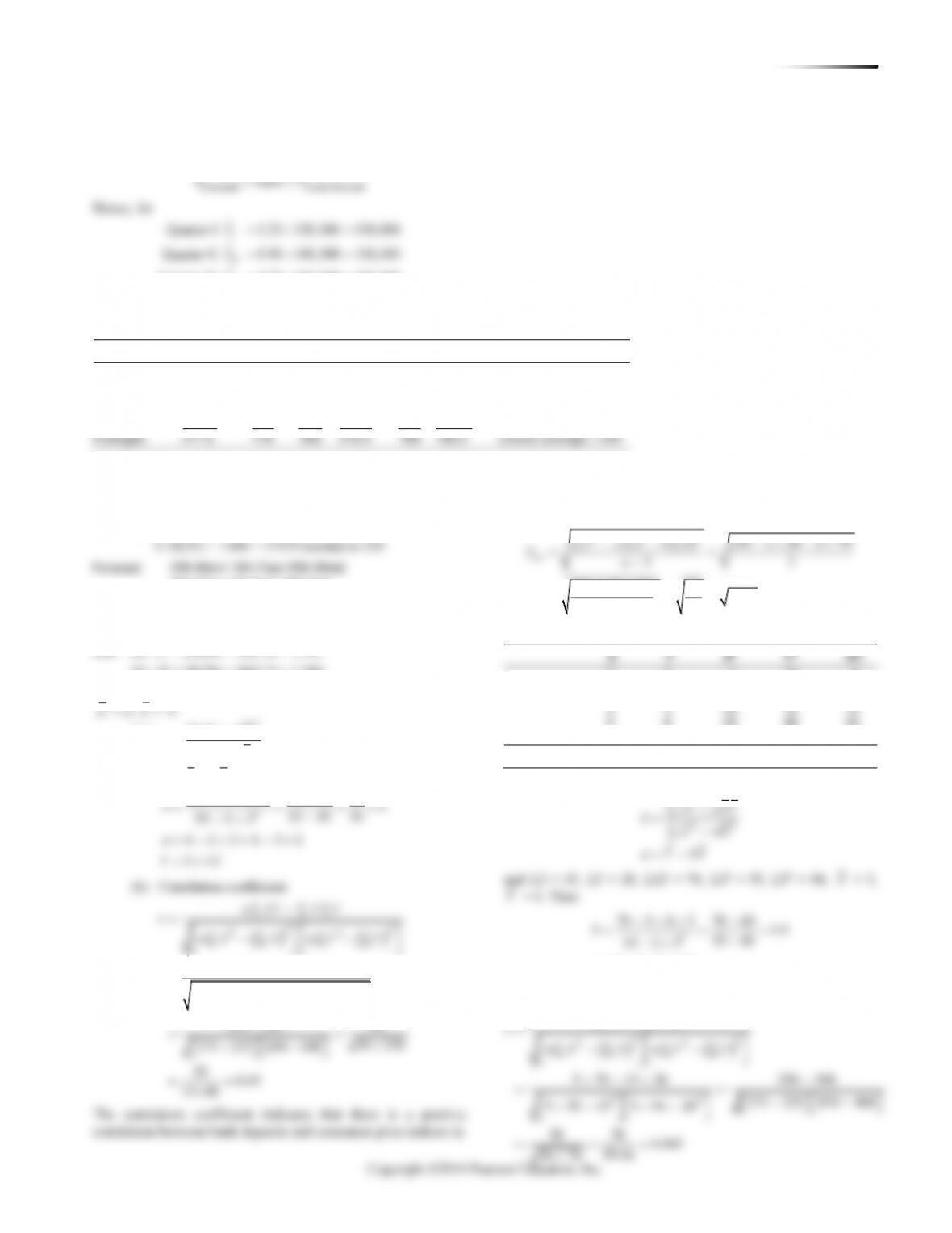
4.55
y
x
x2
xy
7
1
1
7
9
2
4
18
5
3
9
15
11
4
16
44
10
5
25
50
13
6
36
78
55
21
91
212
9.17
3.5
5.27 1.11
y
x
yx
=
=
=+
Period 7 forecast = 13.07
Period 12 forecast = 18.64, but this is far outside the range
of valid data.
Month
Sales
3-Month Moving Average Moving
Absolute Deviation
January
11
February
14
March
16
April
10
(1 × 11 + 2 × 14 + 3 × 16)/6 = 14.50
4.50
May
15
(1 × 14 + 2 × 16 + 3 × 10)/6 = 12.67
2.33
June
17
(1 × 16 + 2 × 10 + 3 × 15)/6 = 13.50
3.50
July
11
(1 × 10 + 2 × 15 + 3 × 17)/6 = 15.17
4.17
August
14
(1 × 15 + 2 × 17 + 3 × 11)/6 = 13.67
0.33
September
17
(1 × 17 + 2 × 11 + 3 × 14)/6 = 13.50
3.50
October
12
(1 × 11 + 2 × 14 + 3 × 17)/6 = 15.00
3.00
November
14
(1 × 14 + 2 × 17 + 3 × 12)/6 = 14.00
0.00
December
16
(1 × 17 + 2 × 12 + 3 × 14)/6 = 13.83
2.17
January
11
(1 × 12 + 2 × 14 + 3 × 16)/6 = 14.67
3.67
February
(1 × 14 + 2 × 16 + 3 × 11)/6 = 13.17
= 27.17
MAD = 2.72
50 CHAPTER 4 FO R E C A S T I N G
1
Standard error of the estimate:
294 1 20 1 70
2 5 2
3
yx
Y a Y b XY
Sn
− − − −
==
−−
= = =
4.62 Using software, the regression equation is: Games lost =
6.41 + 0.533 × days rain.
1. One way to address the case is with separate forecasting models
for each game. Clearly, the homecoming game (week 2) and the
Forecasts
Game
Model
2013
2014
R2
1
y = 30,713 + 2,534x
48,453
50,988
0.92
2
y = 37,640 + 2,146x
52,660
54,806
0.90
3
y = 36,940 + 1,560x
47,860
49,420
0.91
4
y = 22,567 + 2,143x
37,567
39,710
0.88
5
y = 30,440 + 3,146x
52,460
55,606
0.93
2. Revenue in 2013 = (239,000) ($50/ticket) = $11,950,000
Revenue in 2014 = (250,530) ($52.50/ticket) = $13,152,825
3. In games 2 and 5, the forecast for 2014 exceeds stadium ca-
pacity. With this appearing to be a continuing trend, the time has
come for a new or expanded stadium.
VIDEO CASE STUDIES
FORECASTING TICKET REVENUE FOR
6
35
37
1,225
1,369
1,295
7
45
43
2,025
1,849
1,935
8
50
43
2,500
1,849
9
60
54
3,600
2,916
60
66
4,356
3,960
Totals
15,910
15,950
6
35
37
1,225
1,369
1,295
7
45
43
2,025
1,849
1,935
8
50
43
2,500
1,849
9
60
54
3,600
2,916
60
66
4,356
3,960
Totals
15,910
15,950
3. Using the multiple regression model in the case:
Revenue = $14,996 + 10,801 (4) + 23,379 (3) + 10,784 (3)
= $160,743
4. Time of day for game, other competing sports events within
100 miles on that date, special half-time or pregame entertainment
planned, date set for a special group night (for example, Boy
Scouts or Rotary). These may be potential independent variable
for Perez’s model.
cafes, (2) retail sales, (3) banquet sales, (4) concert sales, (5) eval-
uating managers, and (6) menu planning. They could also employ
2. The POS system captures all the basic sales data needed to
drive individual cafe’s scheduling/ordering. It also is aggregated
at corporate HQ. Each entrée sold is counted as one guest at a
3. The weighting system is subjective, but is reasonable. More
weight is given to each of the past 2 years than to 3 years ago.
This system actually protects managers from large sales variations
(weather); hotel occupancy; spring break from colleges; beef pric-
es; promotional budget; etc.
5. Y = a + bx
Month
Advertising X
Guest Count Y
X2
Y2
XY
1
14
21
196
441
294
2
17
24
289
576
408
3
25
27
625
729
675
4
25
32
625
1,024
800
5
35
29
1,225
841
1,015
2
15,910 10 36.6
37.6 0.7996 36.6 8.3363 8.3
8.3363 0.7996
a
YX
−
= − =
=+
At $65,000; y = 8.3 + .8 (65) = 8.3 + 52 = 60.3, or 60,300 guests.
For the instructor who asks other questions than this one:
r2 = 0.8869
Std. error = 5.062
ADDITIONAL CASE STUDIES*
THE NORTH-SOUTH AIRLINE
Northern Airline Data
Airframe Cost
Engine Cost
Average
Year
per Aircraft
per Aircraft
Age (hrs)
2003
51.80
43.49
6512
2004
54.92
38.58
8404
2005
69.70
51.48
11077
2006
68.90
58.72
11717
2007
63.72
45.47
13275
2008
84.73
50.26
15215
2009
78.74
79.60
18390
Southeast Airline Data
Airframe Cost
Engine Cost
Average
Year
per Aircraft
per Aircraft
Age (hrs)
2003
13.29
18.86
5107
2004
25.15
31.55
8145
2005
32.18
40.43
7360
2006
31.78
22.10
5773
2007
25.34
19.69
7150
2008
32.78
32.58
9364
2009
35.56
38.07
8259
Utilizing the software package provided with this text, we
can develop the following regression equations for the variables
of interest:
Northern Airlines—Airframe Maintenance Cost:
www.pearsonhighered.com/heizer and www.myomlab.com.
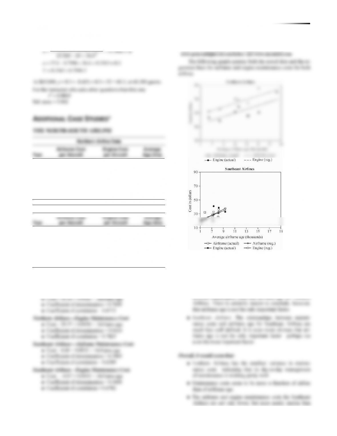
The following graphs portray both the actual data and the re-
gression lines for airframe and engine maintenance costs for both
airlines.
Note that the two graphs have been drawn to the same scale
to facilitate comparisons between the two airlines.
Comparison:
◼ Northern Airlines: There seem to be modest correlations
52 CHAPTER 4 FO R E C A S T I N G
those for Northern Airlines. From the graphs, at least, they
appear to be rising more sharply with age.
From an overall perspective, it appears that Southeast Airlines may
31
627
961
19,437
393,129
32
578
1,024
18,496
334,084
33
585
1,089
19,305
342,225
34
581
1,156
19,754
337,561
35
632
1,225
22,120
399,424
36
656
1,296
23,616
430,336
31
627
961
19,437
393,129
32
578
1,024
18,496
334,084
33
585
1,089
19,305
342,225
34
581
1,156
19,754
337,561
35
632
1,225
22,120
399,424
36
656
1,296
23,616
430,336
1. A plot of the data indicates a linear trend (least squares) mod-
el might be appropriate for forecasting. Using linear trend you
obtain the following:
x
y
x2
xy
y2
1
480
1
480
230,400
2
436
4
872
190,096
3
482
9
1,446
232,324
4
448
16
1,792
200,704
5
458
25
2,290
209,464
6
489
36
2,934
239,121
7
498
49
3,486
248,004
8
430
64
3,440
184,900
9
444
81
3,996
197,136
10
496
100
4,960
246,016
11
487
121
5,357
237,169
12
525
144
6,300
275,625
13
575
169
7,475
330,625
14
527
196
7,378
277,729
15
540
225
8,100
291,600
16
502
256
8,032
252,004
17
508
289
8,636
258,064
18
573
324
10,314
328,329
19
508
361
9,652
258,064
20
498
400
9,960
248,004
22
526
484
11,572
276,676
23
552
529
12,696
304,704
24
587
576
14,088
344,569
15
540
225
8,100
291,600
16
502
256
8,032
252,004
17
508
289
8,636
258,064
18
573
324
10,314
328,329
19
508
361
9,652
258,064
20
498
400
9,960
248,004
22
526
484
11,572
276,676
23
552
529
12,696
304,704
24
587
576
14,088
344,569
25
608
625
15,200
369,664
26
597
676
15,522
356,409
27
612
729
16,524
374,544
28
603
784
16,884
363,609
29
628
841
18,212
394,384
30
605
900
18,150
366,025
440.85 5.25 (time)
y
=+
r = 0.873, indicating a reasonably good fit
The student should report the linear trend results, but deflate
the forecast obtained based upon qualitative information about
industry and technology trends.
Because there is limited seasonality in the data, the linear
trend analysis above provides a good r2 of .76.
However, a more precise forecast can be developed addressing
the seasonality issue, which is done below. Methods a and c yield
r2 of .85 and .86, respectively, and methods b and d, which also
center the seasonal adjustment, yield r2 of .93 and .94, respectively.
2. Four approaches to decomposition of The Digital Cell Phone
data can address seasonality, as follows:
a) Multiplicative seasonal model,
Cases = 443.87 + 5.08 (time), r2 = .85, MAD = 20.89
b) Multiplicative Seasonal Model, with centered moving averages

Copyright ©2014 Pearson Education, Inc.
CHAPTER 4 FO R E C A ST I N G 47
Copyright ©2014 Pearson Education, Inc.
48 CHAPTER 4 FO R E C A S T I N G
4.51
Period
Demand
Exponentially Smoothed Forecast
1
7
5
2
9
5 + 0.2 × (7 – 5) = 5.4
5
13
5.90 + 0.2 × (9 – 5.90) = 6.52
6
8
6.52 + 0.2 × (13 – 6.52) = 7.82
7
Forecast
7.82 + 0.2 × (8 – 7.82) = 7.86
4.52
Actual
Forecast
|Error|
Error2
95
100
5
25
108
110
2
4
123
120
3
9
130
130
0
0
10
38
MAD = 10/4 = 2.5, MSE = 38/4 = 9.5
4.53 (a) 3-month moving average:
3-Month
Absolute
Month
Sales
Moving Average
Deviation
January
11
April
10
(11 + 14 + 16)/3 = 13.67
3.67
May
15
(14 + 16 + 10)/3 = 13.33
1.67
June
17
(16 + 10 + 15)/3 = 13.67
3.33
July
11
(10 + 15 + 17)/3 = 14.00
3.00
August
14
(15 + 17 + 11)/3 = 14.33
0.33
September
17
(17 + 11 + 14)/3 = 14.00
3.00
October
12
(11 + 14 + 17)/3 = 14.00
2.00
November
14
(14 + 17 + 12)/3 = 14.33
0.33
December
16
(17 + 12 + 14)/3 = 14.33
1.67
January
11
(12 + 14 + 16)/3 = 14.00
3.00
February
(14 + 16 + 11)/3 = 13.67
= 22.00
MAD = 2.20
(b) 3-month weighted moving average
(c) Based on a mean absolute deviation criterion, the
3-month moving average with MAD = 2.2 is to be pre-
ferred over the 3-month weighted moving average with
MAD = 2.72.
4.54 (a)
Actual
Cumulative
Cum.
Tracking
Week
Miles
Forecast
Error
Error
|Error|
MAD
Signal
1
17
17.00
0.00
–
0.00
0
2
21
17.00
+4.00
4.00
4.00
2
2
3
19
17.80
+1.20
5.20
5.20
1.73
3
4
23
18.04
+4.96
10.16
10.16
2.54
4
5
18
19.03
–1.03
9.13
11.19
2.24
4
6
16
18.83
–2.83
6.30
14.02
2.34
2.7
7
20
18.26
+1.74
8.04
15.76
2.25
3.6
8
18
18.61
–0.61
7.43
16.37
2.05
3.6
9
22
18.49
+3.51
10.94
19.88
2.21
5
10
20
19.19
+0.81
11.75
20.69
2.07
5.7
11
15
19.35
–4.35
7.40
25.04
2.28
3.2
12
22
18.48
+3.52
10.92
28.56
2.38
4.6
(b) The MAD = 28.56/12 = 2.38
(c) The cumulative error and tracking signals appear to
4.55
y
x
x2
xy
7
1
1
7
9
2
4
18
5
3
9
15
11
4
16
44
10
5
25
50
13
6
36
78
55
21
91
212
9.17
3.5
5.27 1.11
y
x
yx
=
=
=+
Period 7 forecast = 13.07
Period 12 forecast = 18.64, but this is far outside the range
of valid data.
Month
Sales
3-Month Moving Average Moving
Absolute Deviation
January
11
February
14
March
16
April
10
(1 × 11 + 2 × 14 + 3 × 16)/6 = 14.50
4.50
May
15
(1 × 14 + 2 × 16 + 3 × 10)/6 = 12.67
2.33
June
17
(1 × 16 + 2 × 10 + 3 × 15)/6 = 13.50
3.50
July
11
(1 × 10 + 2 × 15 + 3 × 17)/6 = 15.17
4.17
August
14
(1 × 15 + 2 × 17 + 3 × 11)/6 = 13.67
0.33
September
17
(1 × 17 + 2 × 11 + 3 × 14)/6 = 13.50
3.50
October
12
(1 × 11 + 2 × 14 + 3 × 17)/6 = 15.00
3.00
November
14
(1 × 14 + 2 × 17 + 3 × 12)/6 = 14.00
0.00
December
16
(1 × 17 + 2 × 12 + 3 × 14)/6 = 13.83
2.17
January
11
(1 × 12 + 2 × 14 + 3 × 16)/6 = 14.67
3.67
February
(1 × 14 + 2 × 16 + 3 × 11)/6 = 13.17
= 27.17
MAD = 2.72
50 CHAPTER 4 FO R E C A S T I N G
1
Standard error of the estimate:
294 1 20 1 70
2 5 2
3
yx
Y a Y b XY
Sn
− − − −
==
−−
= = =
4.62 Using software, the regression equation is: Games lost =
6.41 + 0.533 × days rain.
1. One way to address the case is with separate forecasting models
for each game. Clearly, the homecoming game (week 2) and the
Forecasts
Game
Model
2013
2014
R2
1
y = 30,713 + 2,534x
48,453
50,988
0.92
2
y = 37,640 + 2,146x
52,660
54,806
0.90
3
y = 36,940 + 1,560x
47,860
49,420
0.91
4
y = 22,567 + 2,143x
37,567
39,710
0.88
5
y = 30,440 + 3,146x
52,460
55,606
0.93
2. Revenue in 2013 = (239,000) ($50/ticket) = $11,950,000
Revenue in 2014 = (250,530) ($52.50/ticket) = $13,152,825
3. In games 2 and 5, the forecast for 2014 exceeds stadium ca-
pacity. With this appearing to be a continuing trend, the time has
come for a new or expanded stadium.
VIDEO CASE STUDIES
FORECASTING TICKET REVENUE FOR
3. Using the multiple regression model in the case:
Revenue = $14,996 + 10,801 (4) + 23,379 (3) + 10,784 (3)
= $160,743
4. Time of day for game, other competing sports events within
100 miles on that date, special half-time or pregame entertainment
planned, date set for a special group night (for example, Boy
Scouts or Rotary). These may be potential independent variable
for Perez’s model.
cafes, (2) retail sales, (3) banquet sales, (4) concert sales, (5) eval-
uating managers, and (6) menu planning. They could also employ
2. The POS system captures all the basic sales data needed to
drive individual cafe’s scheduling/ordering. It also is aggregated
at corporate HQ. Each entrée sold is counted as one guest at a
3. The weighting system is subjective, but is reasonable. More
weight is given to each of the past 2 years than to 3 years ago.
This system actually protects managers from large sales variations
(weather); hotel occupancy; spring break from colleges; beef pric-
es; promotional budget; etc.
5. Y = a + bx
Month
Advertising X
Guest Count Y
X2
Y2
XY
1
14
21
196
441
294
2
17
24
289
576
408
3
25
27
625
729
675
4
25
32
625
1,024
800
5
35
29
1,225
841
1,015
2
15,910 10 36.6
37.6 0.7996 36.6 8.3363 8.3
8.3363 0.7996
a
YX
−
= − =
=+
At $65,000; y = 8.3 + .8 (65) = 8.3 + 52 = 60.3, or 60,300 guests.
For the instructor who asks other questions than this one:
r2 = 0.8869
Std. error = 5.062
ADDITIONAL CASE STUDIES*
THE NORTH-SOUTH AIRLINE
Northern Airline Data
Airframe Cost
Engine Cost
Average
Year
per Aircraft
per Aircraft
Age (hrs)
2003
51.80
43.49
6512
2004
54.92
38.58
8404
2005
69.70
51.48
11077
2006
68.90
58.72
11717
2007
63.72
45.47
13275
2008
84.73
50.26
15215
2009
78.74
79.60
18390
Southeast Airline Data
Airframe Cost
Engine Cost
Average
Year
per Aircraft
per Aircraft
Age (hrs)
2003
13.29
18.86
5107
2004
25.15
31.55
8145
2005
32.18
40.43
7360
2006
31.78
22.10
5773
2007
25.34
19.69
7150
2008
32.78
32.58
9364
2009
35.56
38.07
8259
Utilizing the software package provided with this text, we
can develop the following regression equations for the variables
of interest:
Northern Airlines—Airframe Maintenance Cost:
www.pearsonhighered.com/heizer and www.myomlab.com.
The following graphs portray both the actual data and the re-
gression lines for airframe and engine maintenance costs for both
airlines.
Note that the two graphs have been drawn to the same scale
to facilitate comparisons between the two airlines.
Comparison:
◼ Northern Airlines: There seem to be modest correlations
52 CHAPTER 4 FO R E C A S T I N G
those for Northern Airlines. From the graphs, at least, they
appear to be rising more sharply with age.
From an overall perspective, it appears that Southeast Airlines may
1. A plot of the data indicates a linear trend (least squares) mod-
el might be appropriate for forecasting. Using linear trend you
obtain the following:
x
y
x2
xy
y2
1
480
1
480
230,400
2
436
4
872
190,096
3
482
9
1,446
232,324
4
448
16
1,792
200,704
5
458
25
2,290
209,464
6
489
36
2,934
239,121
7
498
49
3,486
248,004
8
430
64
3,440
184,900
9
444
81
3,996
197,136
10
496
100
4,960
246,016
11
487
121
5,357
237,169
12
525
144
6,300
275,625
13
575
169
7,475
330,625
14
527
196
7,378
277,729
25
608
625
15,200
369,664
26
597
676
15,522
356,409
27
612
729
16,524
374,544
28
603
784
16,884
363,609
29
628
841
18,212
394,384
30
605
900
18,150
366,025
440.85 5.25 (time)
y
=+
r = 0.873, indicating a reasonably good fit
The student should report the linear trend results, but deflate
the forecast obtained based upon qualitative information about
industry and technology trends.
Because there is limited seasonality in the data, the linear
trend analysis above provides a good r2 of .76.
However, a more precise forecast can be developed addressing
the seasonality issue, which is done below. Methods a and c yield
r2 of .85 and .86, respectively, and methods b and d, which also
center the seasonal adjustment, yield r2 of .93 and .94, respectively.
2. Four approaches to decomposition of The Digital Cell Phone
data can address seasonality, as follows:
a) Multiplicative seasonal model,
Cases = 443.87 + 5.08 (time), r2 = .85, MAD = 20.89
b) Multiplicative Seasonal Model, with centered moving averages
Copyright ©2014 Pearson Education, Inc.