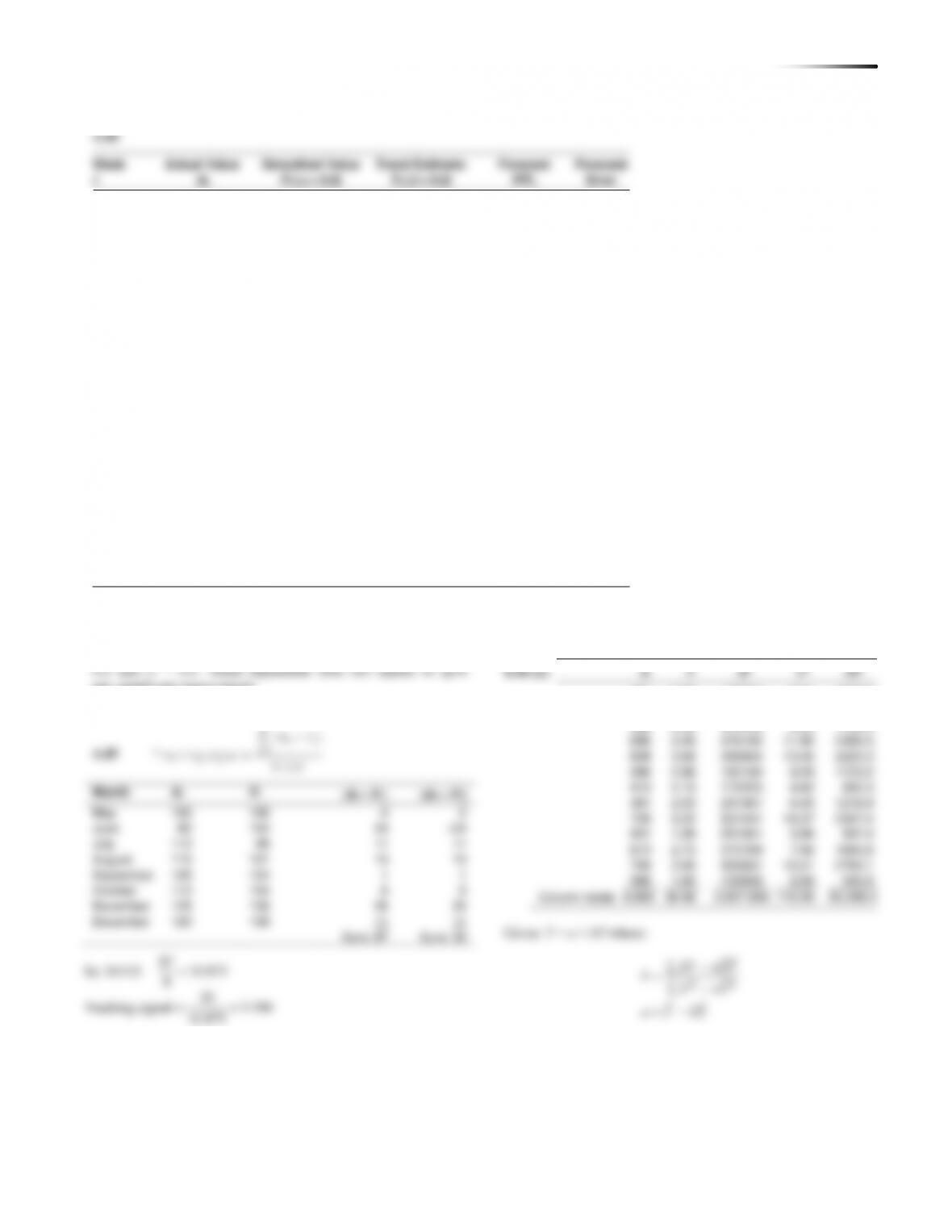
38 CHAPTER 4 FO R E C A S T I N G
Quarter
Number
Winter
101
120.43
Spring
102
120.86
1.1
132.946
Summer
103
121.29
1.4
169.806
Fall
104
121.72
16
256
12
144
18
324
14
196
Error
1
–4
2
–2
3
4
2
5
–6
Totals
15
3
Copyright ©2014 Pearson Education, Inc.
4.34 Y = 7.5 + 3.5X1 + 4.5X2 + 2.5X3
(a) 28
(b) 43
4.35 (a)
ˆ
Y
= 13,473 + 37.65(1860) = 83,502
(b) The predicted selling price is $83,502, but this is the
1
36
1
1,296
36
2
33
4
1,089
66
3
40
9
1,600
120
4
41
16
1,681
164
5
40
25
1,600
200
6
55
36
3,025
330
7
60
49
3,600
8
54
64
2,916
432
1
36
1
1,296
36
2
33
4
1,089
66
3
40
9
1,600
120
4
41
16
1,681
164
5
40
25
1,600
200
6
55
36
3,025
330
7
60
49
3,600
8
54
64
2,916
432
4.36 (a) Given: Y = 90 + 48.5X1 + 0.4X2 where:
1
2
expected travel cost
number of days on the road
distance traveled, in miles
0.68 (coefficient of correlation)
Y
X
X
r
=
=
=
=
If:
Number of days on the road → X1 = 5 and distance
traveled → X2 = 300
then:
Y = 90 + 48.5 × 5 + 0.4 × 300 = 90 + 242.5 + 120 = 452.5
Therefore, the expected cost of the trip is $452.50.
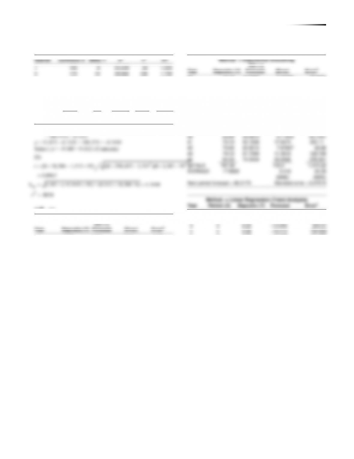
(c) A number of other variables should be included, such as:
Period
Demand
Forecast
Error
Running Sum
|Error|
1
20
20
0.00
0.00
0.00
2
21
20
1.00
1.00
1.00
3
28
20.5
7.50
8.50
7.50
6
29
27.81
1.19
16.82
1.19
7
36
28.41
7.59
24.41
7.59
8
22
32.20
–10.20
14.21
10.20
9
25
27.11
–2.10
12.10
2.10
10
28
26.05
1.95
14.05
1.95
MAD
5.00
Cumulative error = 14.05; MAD = 5 Tracking = 14.05/5 = 2.82
9
58
81
3,364
522
10
61
100
3,721
610
55
478
385
23,892
2,900
Given: Y = a + bX where:
22
XY nXY
b
X nX
a Y bX
−
=−
=−
and X = 55, Y = 478, XY = 2900, X2 = 385, Y2 = 23892,
5.5, 47.8,XY==
Then:
− −
= = = =
2,900 10 5.5 47.8 2,900 2,629 271 3.28
b
11: 29.76 3.28 11 65.8
XY
= = + =
4
37
24.25
21.25
5
25
30.63
–5.63
15.63
5.63
4
37
24.25
21.25
5
25
30.63
–5.63
15.63
5.63
40 CHAPTER 4 FO R EC A S T I N G
()()
−
=
− −
−
=
− −
−
10
29.8 + 3.28 × 10 = 62.6
12
11.9
10
29.8 + 3.28 × 10 = 62.6
12
11.9
22
22
22
10 2900 55 478
10 385 55 10 23892 478
29000 26290
n XY X Y
r
n X X n Y Y
Column totals
854.0
478
76,129.9
23,892
42,558.6
Given: Y = a + bX where
22
XY nXY
b
X nX
a Y bX
−
=−
=−
and X = 854, Y = 478, XY = 42558.6, X2 = 76129.9,

42 CHAPTER 4 FO R EC A S T I N G
(f) The correlation coefficient and the coefficient of deter-
+50.0
+50.0
+41.0
+31.4
+36.6
+41.6
+37.6
+27.1
+28.8
10
+32.5
11
+25.0
12
+19.0
13
+31.6
14
+45.6
15
+39.3
16
+30.7
17
+45.3
18
+51.1
19
+44.4
20
+38.8
21
+51.5
22
+65.6
23
+56.2
24
+46.5
+50.0
+50.0
+41.0
+31.4
+36.6
+41.6
+37.6
+27.1
+28.8
10
+32.5
11
+25.0
12
+19.0
13
+31.6
14
+45.6
15
+39.3
16
+30.7
17
+45.3
18
+51.1
19
+44.4
20
+38.8
21
+51.5
22
+65.6
23
+56.2
24
+46.5
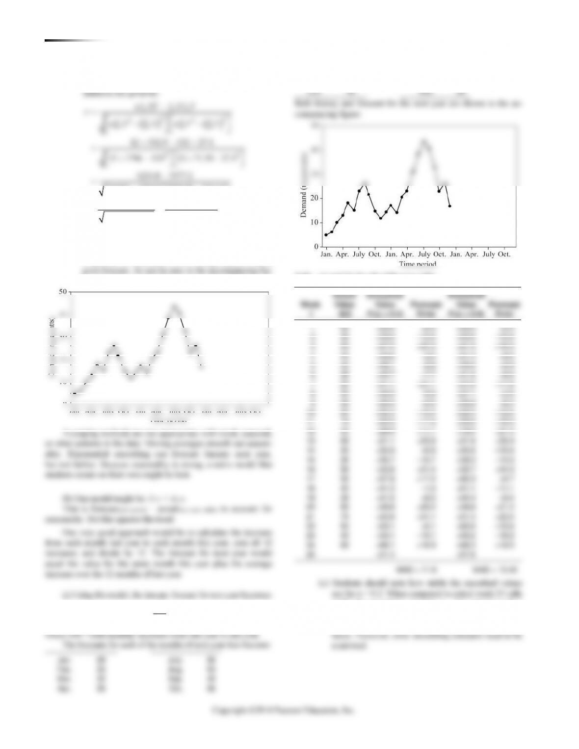
Jan.
29
July.
56
Jan.
29
July.
56
Feb.
26
Aug.
53
Mar.
32
Sep.
45
Apr.
35
Oct.
35
May.
42
Nov.
38
Copyright ©2014 Pearson Education, Inc.
0.2 and = 0.6. Trend adjustment does not appear to give
any significant improvement.
4.45
Month
At
Ft
|At – Ft |
(At – Ft)
May
100
100
0
0
June
80
104
24
–24
July
110
99
11
11
August
115
101
14
14
September
105
104
1
1
October
110
104
6
6
November
125
105
20
20
December
120
109
11
11
Sum: 87
Sum: 39
4.46 (a)
X
Y
X2
Y2
XY
421
2.90
177241
8.41
1220.9
377
2.93
142129
8.58
1104.6
585
3.00
342225
9.00
1755.0
690
3.45
476100
11.90
2380.5
608
3.66
369664
13.40
2225.3
390
2.88
152100
8.29
1123.2
415
2.15
172225
4.62
892.3
481
2.53
231361
6.40
1216.9
729
3.22
531441
10.37
2347.4
501
1.99
251001
3.96
997.0
613
2.75
375769
7.56
1685.8
709
3.90
502681
15.21
2765.1
366
1.60
133956
2.56
585.6
Column totals
6,885
36.96
3,857,893
110.26
20,299.5
Given: Y = a + bX where:
22
XY nXY
b
X nX
a Y bX
−
=−
=−
()
Tracking signal M A D
n
tt
t
AF
=
−
=1
=
==
87
So: MAD: 10.875
8
39
Tracking signal 3.586
10.875
1
2
3
4
5
6
7
8
9
1
2
3
4
5
6
7
8
9
44 CHAPTER 4 FO R EC A S T I N G
and X = 6885, Y = 36.96, XY = 20299.5, X2 = 3857893,
Y2 = 110.26,
X
= 529.6,
Y
= 2.843. Then:
2
20299.5 13 529.6 2.843 20299.5 19573.5
3857893 3646190
3857893 13 529.6
726 0.0034
211703
2.84 0.0034 529.6 1.03
b
a
− −
==
−
−
==
= − =
and Y = 1.03 + 0.0034X
As an indication of the usefulness of this relationship, we can
calculate the correlation coefficient:
()()
22
22
22
13 20299.5 6885 36.96
13 3857893 6885 13 110.26 36.96
263893.5 254469.6
50152609 47403225 1433.4 1366.0
9423.9
2749384 67.0
9423.9 0.69
1658.13 8.21
n XY X Y
r
n X X n Y Y
−
=
− −
−
=
− −
−
=−−
=
==
2
2
0.479r=
A correlation coefficient of 0.692 is not particularly high. The
coefficient of determination, r2, indicates that the model explains
only 47.9% of the overall variation. Therefore, while the model
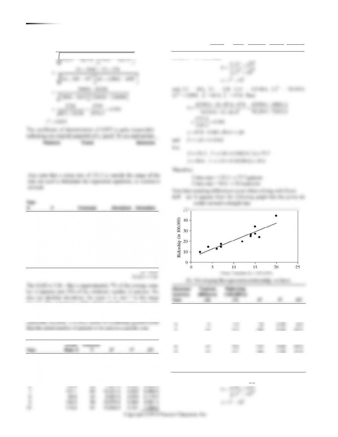
4.47 (a) There is not a strong linear trend in sales over time.
(b, c) Bob wants to forecast by exponential smoothing (setting
February’s forecast equal to January’s sales) with alpha =
0.1. Sherry wants to use a 3-period moving average.
Sales
Bob
Sherry
Bob’s Error
Sherry’s Error
January
400
—
—
—
—
February
380
400
—
20.0
—
March
410
398
—
12.0
—
April
375
24.2
May
405
March
410
398
—
12.0
—
April
375
24.2
May
405
Bob’s MAD for exponential smoothing (16.11) is lower than
that of Sherry’s moving average (19.17). So his forecast
seems to be better.
Copyright ©2014 Pearson Education, Inc.
4.34 Y = 7.5 + 3.5X1 + 4.5X2 + 2.5X3
(a) 28
(b) 43
4.35 (a)
ˆ
Y
= 13,473 + 37.65(1860) = 83,502
(b) The predicted selling price is $83,502, but this is the
4.36 (a) Given: Y = 90 + 48.5X1 + 0.4X2 where:
1
2
expected travel cost
number of days on the road
distance traveled, in miles
0.68 (coefficient of correlation)
Y
X
X
r
=
=
=
=
If:
Number of days on the road → X1 = 5 and distance
traveled → X2 = 300
then:
Y = 90 + 48.5 × 5 + 0.4 × 300 = 90 + 242.5 + 120 = 452.5
Therefore, the expected cost of the trip is $452.50.
(c) A number of other variables should be included, such as:
Period
Demand
Forecast
Error
Running Sum
|Error|
1
20
20
0.00
0.00
0.00
2
21
20
1.00
1.00
1.00
3
28
20.5
7.50
8.50
7.50
6
29
27.81
1.19
16.82
1.19
7
36
28.41
7.59
24.41
7.59
8
22
32.20
–10.20
14.21
10.20
9
25
27.11
–2.10
12.10
2.10
10
28
26.05
1.95
14.05
1.95
MAD
5.00
Cumulative error = 14.05; MAD = 5 Tracking = 14.05/5 = 2.82
9
58
81
3,364
522
10
61
100
3,721
610
55
478
385
23,892
2,900
Given: Y = a + bX where:
22
XY nXY
b
X nX
a Y bX
−
=−
=−
and X = 55, Y = 478, XY = 2900, X2 = 385, Y2 = 23892,
5.5, 47.8,XY==
Then:
− −
= = = =
2,900 10 5.5 47.8 2,900 2,629 271 3.28
b
11: 29.76 3.28 11 65.8
XY
= = + =
40 CHAPTER 4 FO R EC A S T I N G
()()
−
=
− −
−
=
− −
−
22
22
22
10 2900 55 478
10 385 55 10 23892 478
29000 26290
n XY X Y
r
n X X n Y Y
Column totals
854.0
478
76,129.9
23,892
42,558.6
Given: Y = a + bX where
22
XY nXY
b
X nX
a Y bX
−
=−
=−
and X = 854, Y = 478, XY = 42558.6, X2 = 76129.9,
42 CHAPTER 4 FO R EC A S T I N G
(f) The correlation coefficient and the coefficient of deter-
Feb.
26
Aug.
53
Mar.
32
Sep.
45
Apr.
35
Oct.
35
May.
42
Nov.
38
Copyright ©2014 Pearson Education, Inc.
0.2 and = 0.6. Trend adjustment does not appear to give
any significant improvement.
4.45
Month
At
Ft
|At – Ft |
(At – Ft)
May
100
100
0
0
June
80
104
24
–24
July
110
99
11
11
August
115
101
14
14
September
105
104
1
1
October
110
104
6
6
November
125
105
20
20
December
120
109
11
11
Sum: 87
Sum: 39
4.46 (a)
X
Y
X2
Y2
XY
421
2.90
177241
8.41
1220.9
377
2.93
142129
8.58
1104.6
585
3.00
342225
9.00
1755.0
690
3.45
476100
11.90
2380.5
608
3.66
369664
13.40
2225.3
390
2.88
152100
8.29
1123.2
415
2.15
172225
4.62
892.3
481
2.53
231361
6.40
1216.9
729
3.22
531441
10.37
2347.4
501
1.99
251001
3.96
997.0
613
2.75
375769
7.56
1685.8
709
3.90
502681
15.21
2765.1
366
1.60
133956
2.56
585.6
Column totals
6,885
36.96
3,857,893
110.26
20,299.5
Given: Y = a + bX where:
22
XY nXY
b
X nX
a Y bX
−
=−
=−
()
Tracking signal M A D
n
tt
t
AF
=
−
=1
=
==
87
So: MAD: 10.875
8
39
Tracking signal 3.586
10.875
44 CHAPTER 4 FO R EC A S T I N G
and X = 6885, Y = 36.96, XY = 20299.5, X2 = 3857893,
Y2 = 110.26,
X
= 529.6,
Y
= 2.843. Then:
2
20299.5 13 529.6 2.843 20299.5 19573.5
3857893 3646190
3857893 13 529.6
726 0.0034
211703
2.84 0.0034 529.6 1.03
b
a
− −
==
−
−
==
= − =
and Y = 1.03 + 0.0034X
As an indication of the usefulness of this relationship, we can
calculate the correlation coefficient:
()()
22
22
22
13 20299.5 6885 36.96
13 3857893 6885 13 110.26 36.96
263893.5 254469.6
50152609 47403225 1433.4 1366.0
9423.9
2749384 67.0
9423.9 0.69
1658.13 8.21
n XY X Y
r
n X X n Y Y
−
=
− −
−
=
− −
−
=−−
=
==
2
2
0.479r=
A correlation coefficient of 0.692 is not particularly high. The
coefficient of determination, r2, indicates that the model explains
only 47.9% of the overall variation. Therefore, while the model
4.47 (a) There is not a strong linear trend in sales over time.
(b, c) Bob wants to forecast by exponential smoothing (setting
February’s forecast equal to January’s sales) with alpha =
0.1. Sherry wants to use a 3-period moving average.
Sales
Bob
Sherry
Bob’s Error
Sherry’s Error
January
400
—
—
—
—
February
380
400
—
20.0
—
Bob’s MAD for exponential smoothing (16.11) is lower than
that of Sherry’s moving average (19.17). So his forecast
seems to be better.