
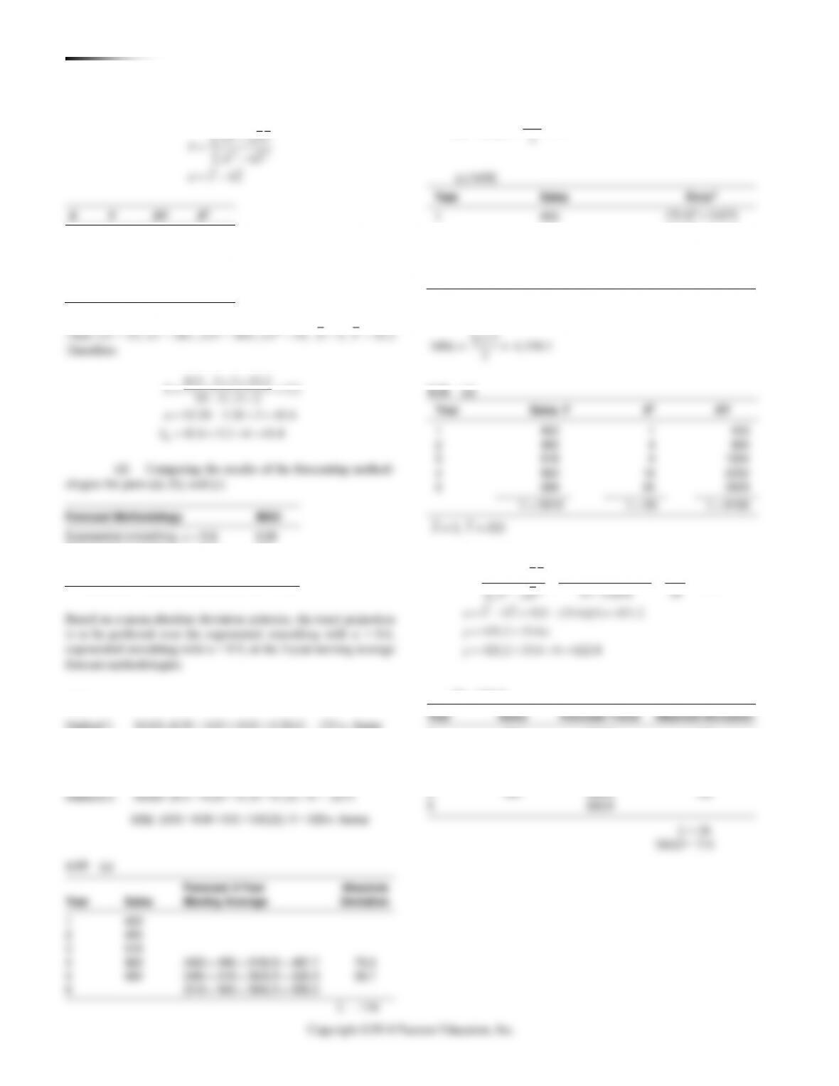
30 CHAPTER 4 FO R E C A ST I N G
(d) The 3-year moving average appears to give better
results.
Year
Mileage
|Error|
1
3,000
2
4,000
3
3,400
100
4
3,800
100
5
3,700
100
100
Totals
100
January
February
4
April
16
May
25
June
36
July
49
August
64
September
81
October
100
November
121
Sum
218
650
1,474
Year
Mileage
|Error|
1
3,000
2
4,000
3
3,400
100
4
3,800
100
5
3,700
100
100
Totals
100
January
February
4
April
16
May
25
June
36
July
49
August
64
September
81
October
100
November
121
Sum
218
650
1,474
4.5 (c) Weighted 2-year M.A. with .6 weight for most recent year.
Year
Mileage
Forecast
Error
|Error|
1
3,000
2
4,000
3
3,400
3,600
–200
200
4
3,800
3,640
160
160
5
3,700
3,640
60
60
420
Forecast for year 6 is 3,740 miles.
420
MAD 140 3
==
4.5 (d)
Year
Mileage
Forecast
Forecast
Error
Error ×
= .50
New
Forecast
1
3,000
3,000
0
0
3,000
2
4,000
3,000
1,000
500
3,500
3
3,400
3,500
–100
–50
3,450
4
3,800
3,450
350
175
3,625
5
3,700
3,625
75
38
3,663
Total
1,325
The forecast is 3,663 miles.
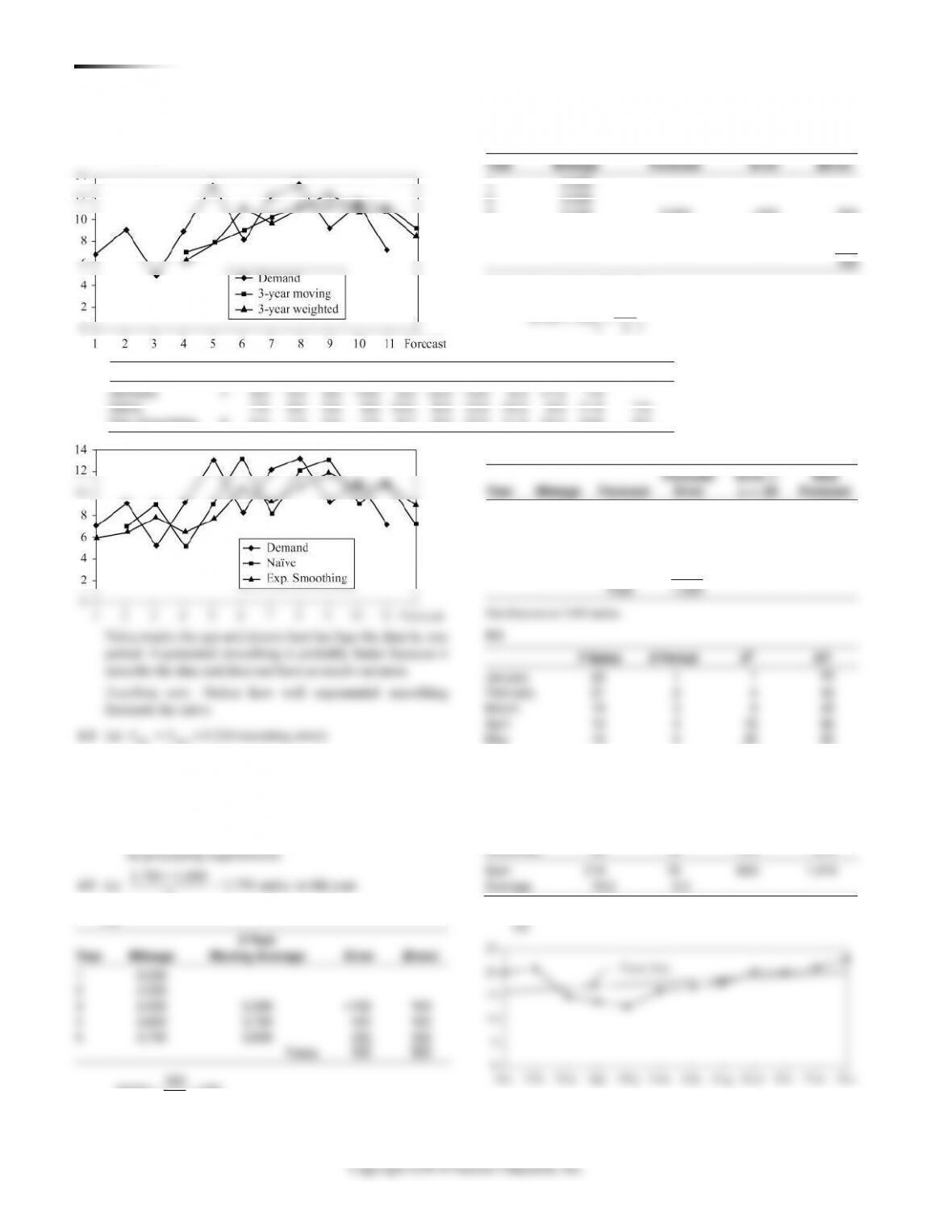
4.3
Year
1
2
3
4
5
6
7
8
9
10
11
Forecast
Demand
7
9.0
5.0
9.0
13.0
8.0
12.0
13.0
9.0
11.0
7.0
Naïve
7.0
9.0
5.0
9.0
13.0
8.0
12.0
13.0
9.0
11.0
7.0
Exp. Smoothing
6
6.4
7.4
6.5
7.5
9.7
9.0
10.2
11.3
10.4
10.6
9.2
CHAPTER 4 FO R E C A S T I N G 31
(b) [i] Naïve The coming January = December = 23
[ii] 3-month moving (20 + 21 + 23)/3 = 21.33
++ =
(96 88 90)
(a) 91.3
3
4.8
+=
(88 90)
32 CHAPTER 4 FO R E C A ST I N G
4.11
Year
1
2
3
4
5
6
7
8
9
10
11
Forecast
Demand
4
6.0
4.0
5.0
10.0
8.0
7.0
9.0
12.0
14.0
15.0
Exp. smoothing
4.7
5.1
4.8
4.8
6.4
6.9
6.9
7.5
8.9
10.4
4.11
Year
1
2
3
4
5
6
7
8
9
10
11
Forecast
Demand
4
6.0
4.0
5.0
10.0
8.0
7.0
9.0
12.0
14.0
15.0
Exp. smoothing
4.7
5.1
4.8
4.8
6.4
6.9
6.9
7.5
8.9
10.4
4.9
(d) Table for Problem 4.9(d):
= .1
= .3
= .5
Month
Price per Chip
Forecast
|Error|
Forecast
|Error|
Forecast
|Error|
January
$1.80
$1.80
$.00
$1.80
$.00
$1.80
$.00
February
1.67
1.80
.13
1.80
.13
1.80
.13
March
1.70
1.79
.09
1.76
.06
1.74
.04
April
1.85
1.78
.07
1.74
.11
1.72
.13
May
1.90
1.79
.11
1.77
.13
1.78
.12
June
1.87
1.80
.07
1.81
.06
1.84
.03
July
1.80
1.80
.00
1.83
.03
1.86
.06
August
1.83
1.80
.03
1.82
.01
1.83
.00
September
1.70
1.81
.11
1.82
.12
1.83
.13
October
1.65
1.80
.15
1.79
.14
1.76
.11
November
1.70
1.78
.08
1.75
.05
1.71
.01
December
1.75
1.77
.02
1.73
.02
1.70
.05
Totals
$.86
$.86
$.81
MAD (total/12)
$.072
$.072
$.0675
= .5 is preferable, using MAD, to = .1 or = .3. One could
also justify excluding the January error and then dividing by
n = 11 to compute the MAD. These numbers would be $.078
(for = .1), $.078 (for = .3), and $.074 (for = .5).
4.10
Year
1
2
3
4
5
6
7
8
9
10
11
Forecast
Demand
4
6
4
5.0
10.0
8.0
7.0
9.0
12.0
14.0
15.0
(a)
3-year moving
4.7
5.0
6.3
7.7
8.3
8.0
9.3
11.7
13.7
(b)
3-year weighted
4.5
5.0
7.3
7.8
8.0
8.3
10.0
12.3
14.0

CHAPTER 4 FO R E C A S T I N G 33
2
Error 104.87
4.12
t
Day
Actual
Demand
Forecast
Demand
1
Monday
88
88
2
Tuesday
72
88
3
Wednesday
68
84
4
Thursday
48
80
5
Friday
1
2
3
4
5
6
Year
Deviation
3
4
5
6
Year
Deviation
1
2
3
4
5
4
Thursday
48
80
5
Friday
1
2
3
4
5
6
Year
Deviation
3
4
5
6
Year
Deviation
1
2
3
4
5
1
2
1
2
Year
Demand
Smoothing = 0.9
Deviation
1
45
41
4.0
2
50
41.0 + 0.9(45–41) = 44.6
5.4
3
52
44.6 + 0.9(50–44.6 ) = 49.5
2.5
4
56
49.5 + 0.9(52–49.5) = 51.8
4.2
5
58
51.8 + 0.9(56–51.8) = 55.6
2.4
6
?
55.6 + 0.9(58–55.6) = 57.8
= 18.5
MAD = 3.7
(b) |Error| = |Actual – Forecast|
Year
1
2
3
4
5
6
7
8
9
10
11
MAD
Exp. Smoothing error
1
1.3
1.1
0.2
5.2
1.6
0.1
2.1
4.5
5.1
4.6
2.4
These calculations were completed in Excel. Calculations are slightly different in Excel OM and POM for Windows due to
rounding differences.
34 CHAPTER 4 FO R E C A ST I N G
=+
=
22
–
–
Y a bX
XY nXY
b
X nX
(b)
134
MAD 67
2
==
Copyright ©2014 Pearson Education, Inc.
164.4
164.4
M SE 32.88
5
=
==
4.17
Forecast Exponential
Absolute
Year
Sales
Smoothing = 0.6
Deviation
1
450
410.0
40.0
2
495
410 + 0.6(450 – 410) = 434.0
61.0
3
518
434 + 0.6(495 – 434) = 470.6
47.4
4
563
470.6 + 0.6(518 – 470.6) = 499.0
64.0
5
584
499 + 0.6(563 – 499) = 537.4
46.6
Year
4
563
470.6 + 0.6(518 – 470.6) = 499.0
64.0
5
584
499 + 0.6(563 – 499) = 537.4
46.6
Year
1
450
410.0
40.0
2
495
410 + 0.9(450 – 410) = 446.0
49.0
3
518
446 + 0.9(495 – 446) = 490.1
27.9
4
563
490.1 + 0.9(518 – 490.1) = 515.2
47.8
5
584
515.2 + 0.9(563 – 515.2) = 558.2
25.8
6
558.2 + 0.9(584 – 558.2) = 581.4
= 190.5
MAD = 38.1
(Refer to Solved Problem 4.1)
For = 0.3, absolute deviations for years 1–5 are 40.0, 73.0, 74.1,
0.6
0.9
MAD 51.8
MAD 38.1
=
=
=
=
Because it gives the lowest MAD, the smoothing constant of
= 0.9 gives the most accurate forecast.
50 + (50 – 50) holds for any ). Let’s pick t = 3. Then F3 = 48 =
50 + (42 – 50)
or 48 = 50 + 42 – 50
or –2 = –8
So, .25 =
4.19 Trend adjusted exponential smoothing: = 0.1, = 0.2
Unadjusted
Adjusted
Month
Income
Forecast
Trend
Forecast
|Error|
Error2
February
70.0
65.0
0.0
65
5.0
25.0
March
68.5
65.5
0.1
65.6
2.9
8.4
April
64.8
65.9
0.16
66.05
1.2
1.6
May
71.7
65.92
0.13
66.06
5.6
31.9
June
71.3
66.62
0.25
66.87
4.4
19.7
July
72.8
67.31
0.33
67.64
5.2
26.6
August
68.16
68.60
24.3
113.2
MAD = 24.3/6 = 4.05, MSE = 113.2/6 = 18.87. Note that all
numbers are rounded.
36 CHAPTER 4 FO R E C A ST I N G
Unadjusted
Adjusted
Month
Demand (y)
Forecast
Trend
Forecast
Error
|Error|
Error2
February
70.0
65.0
0
65.0
5.00
5.0
25.00
March
68.5
65.5
0.4
65.9
2.60
2.6
6.76
April
64.8
66.16
0.61
66.77
–1.97
1.97
3.87
May
71.7
66.57
0.45
67.02
4.68
4.68
21.89
June
71.3
67.49
0.82
68.31
2.99
2.99
8.91
July
72.8
68.61
1.06
69.68
3.12
3.12
9.76
Totals
419.1
16.42
20.36
76.19
Average
69.85
2.74
3.39
12.70
August forecast
71.30
(Bias)
(MAD)
(MSE)
Based upon the MSE criterion, the exponential smoothing with = 0.1, = 0.8 is to be preferred
over the exponential smoothing with = 0.1, = 0.2. Its MSE of 12.70 is lower. Its MAD of 3.39 is
also lower than that in Problem 4.19.
4.20 Trend adjusted exponential smoothing: = 0.1, = 0.8
( )
( )
( )( ) ( )( )
5 4 4 4
1 – 0.2 19 0.8 20.14
3.8 16.11 19.91
F A F T4.21 = + + = +
= + =
()
( ) ( )( )
( )( ) ( )
5 5 4 4
– 1 – 0.4 19.91 – 17.82
0.6 2.32 0.4 2.09
1.39 0.84 1.39 2.23
T F F T= + =
+=
+ = + =
5 5 5 19.91 2.23 22.14FIT F T= + = + =
( )
()
( )( ) ( )( )
6 5 5 5
1 – 0.2 24 0.8 22.14
4.8 17.71 22.51
F A F T= + + = +
= + =
()
( ) ( ) ( )
( )
6 6 5 5
– 1 – 0.4 22.51 – 19.91 0.6 2.23
0.4 2.6 1.34
1.04 1.34 2.38
T F F T= + = +
=+
= + =
6 6 6 22.51 2.38 24.89FIT F T= + = + =
7 6 6 6
7 7 6 6
7 7 7
(1 – )( ) (0.2)(21) (0.8)(24.89)
4.2 19.91 24.11
( – ) (1 – ) (0.4)(24.11 – 22.51)
(0.6)(2.38) 2.07
24.11 2.07 26.18
F A F T
T F F T
FIT F T
4.22 = + + = +
= + =
= + =
+=
= + = + =
8 7 7 7
(1 – )( ) (0.2)(31)
F A F T= + + =
()
( ) ( )
( )
8 8 7 7
– 1 – 0.4 27.14 – 24.11
0.6 2.07 2.45
T F F T= + =
+=
( )
()
( )( )
( )( )
8 8 8
9 8 8 8
27.14 2.45 29.59
1 – 0.2 28
0.8 29.59 29.28
FIT F T
F A F T
= + = + =
= + + =
+=
()
( ) ( )( )
( )( )
9 9 8 8
– 1 – 0.4 29.28 – 27.14
0.6 2.45 2.32
T F F T= + =
+=
9 9 9 29.28 2.32 31.60FIT F T= + = + =
4.23 Students must determine the naïve forecast for the four
months. The naïve forecast for March is the February actual of 83,
etc.
(a)
Actual
Forecast
|Error|
|% Error|
March
101
120
19
100 (19/101) = 18.81%
April
96
114
18
100 (18/96) = 18.75%
May
89
110
21
100 (21/89) = 23.60%
June
108
108
0
100 (0/108) = 0%
58
61.16%
58
MAD (for management) 14.5
4
61.16%
MAPE (for management) 15.29%
4
==
==
(b)
Actual
Naïve
|Error|
|% Error|
March
101
83
18
100 (18/101) = 17.82%
April
96
101
5
100 (5/96) = 5.21%
May
89
96
7
100 (7/89) = 7.87%
June
108
89
19
100 (19/108) = 17.59%
49
48.49%
==
==
49
MAD (for naïve) 12.25
4
48.49%
MAPE (for naïve) 12.12%
4
Naïve outperforms management.
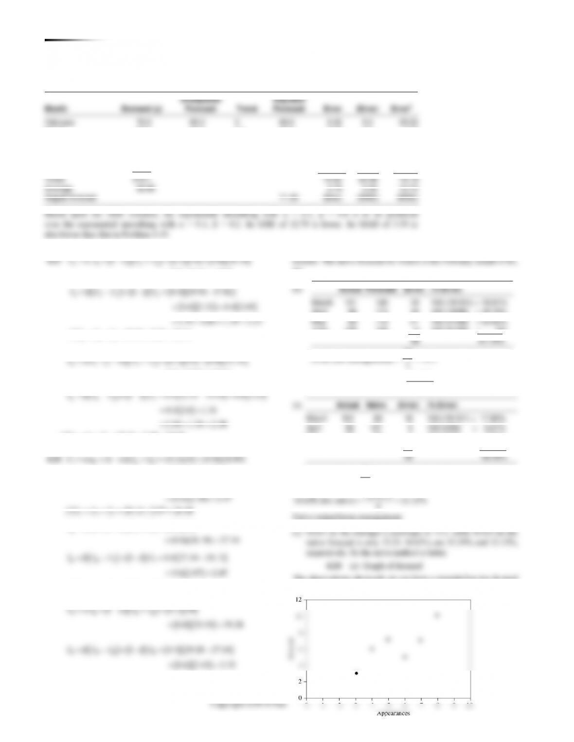
4.24 (a) Graph of demand
The observations obviously do not form a straight line but do tend
to cluster about a straight line over the range shown.
CHAPTER 4 FO R E C A S T I N G 37
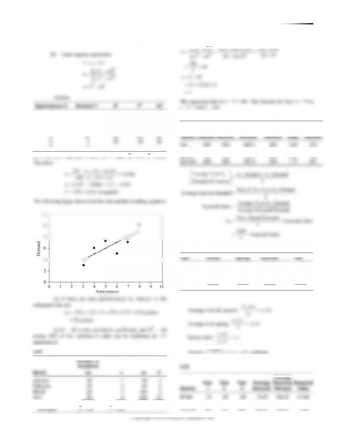
(b) Least-squares regression:
22
Y a bX
XY nXY
b
X nX
a Y bX
=+
−
=−
=−
Assume
Appearances X
Demand Y
X2
Y2
XY
3
3
9
9
9
4
6
16
36
24
7
7
49
49
49
6
5
36
25
30
8
10
64
100
80
5
7
25
49
35
9
?
2 2 2
650 4(2.5)(55) 650 550
30 25
30 4(2.5)
100 20
5
55 (20)(2.5)
5
xy n x y
b
x nx
a y bx
− − −
= = = −
− −
==
=−
=−
=
The regression line is y = 5 + 20x. The forecast for May (x = 5) is
y = 5 + 20(5) = 105.
4.26
Season
Year1
Demand
Year2
Demand
Average
Year1–Year2
Demand
Average
Season
Demand
Seasonal
Index
Year3
Demand
Fall
200
250
225.0
250
0.90
270
Winter
350
300
325.0
250
1.30
390
Accidents
January
Spring
150
165
157.5
250
0.63
189
1
1,400
2
1,200
3
1,000
4
4,500
Winter
Accidents
January
Spring
150
165
157.5
250
0.63
189
1
1,400
2
1,200
3
1,000
4
4,500
Winter
30 CHAPTER 4 FO R E C A ST I N G
(d) The 3-year moving average appears to give better
results.
4.5 (c) Weighted 2-year M.A. with .6 weight for most recent year.
Year
Mileage
Forecast
Error
|Error|
1
3,000
2
4,000
3
3,400
3,600
–200
200
4
3,800
3,640
160
160
5
3,700
3,640
60
60
420
Forecast for year 6 is 3,740 miles.
420
MAD 140 3
==
4.5 (d)
Year
Mileage
Forecast
Forecast
Error
Error ×
= .50
New
Forecast
1
3,000
3,000
0
0
3,000
2
4,000
3,000
1,000
500
3,500
3
3,400
3,500
–100
–50
3,450
4
3,800
3,450
350
175
3,625
5
3,700
3,625
75
38
3,663
Total
1,325
The forecast is 3,663 miles.
4.3
Year
1
2
3
4
5
6
7
8
9
10
11
Forecast
Demand
7
9.0
5.0
9.0
13.0
8.0
12.0
13.0
9.0
11.0
7.0
Naïve
7.0
9.0
5.0
9.0
13.0
8.0
12.0
13.0
9.0
11.0
7.0
Exp. Smoothing
6
6.4
7.4
6.5
7.5
9.7
9.0
10.2
11.3
10.4
10.6
9.2
CHAPTER 4 FO R E C A S T I N G 31
(b) [i] Naïve The coming January = December = 23
[ii] 3-month moving (20 + 21 + 23)/3 = 21.33
++ =
(96 88 90)
(a) 91.3
3
4.8
+=
(88 90)
32 CHAPTER 4 FO R E C A ST I N G
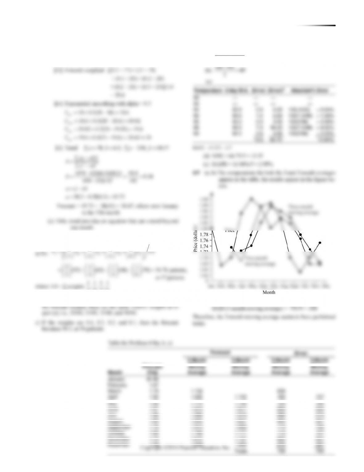
4.9
(d) Table for Problem 4.9(d):
= .1
= .3
= .5
Month
Price per Chip
Forecast
|Error|
Forecast
|Error|
Forecast
|Error|
January
$1.80
$1.80
$.00
$1.80
$.00
$1.80
$.00
February
1.67
1.80
.13
1.80
.13
1.80
.13
March
1.70
1.79
.09
1.76
.06
1.74
.04
April
1.85
1.78
.07
1.74
.11
1.72
.13
May
1.90
1.79
.11
1.77
.13
1.78
.12
June
1.87
1.80
.07
1.81
.06
1.84
.03
July
1.80
1.80
.00
1.83
.03
1.86
.06
August
1.83
1.80
.03
1.82
.01
1.83
.00
September
1.70
1.81
.11
1.82
.12
1.83
.13
October
1.65
1.80
.15
1.79
.14
1.76
.11
November
1.70
1.78
.08
1.75
.05
1.71
.01
December
1.75
1.77
.02
1.73
.02
1.70
.05
Totals
$.86
$.86
$.81
MAD (total/12)
$.072
$.072
$.0675
= .5 is preferable, using MAD, to = .1 or = .3. One could
also justify excluding the January error and then dividing by
n = 11 to compute the MAD. These numbers would be $.078
(for = .1), $.078 (for = .3), and $.074 (for = .5).
4.10
Year
1
2
3
4
5
6
7
8
9
10
11
Forecast
Demand
4
6
4
5.0
10.0
8.0
7.0
9.0
12.0
14.0
15.0
(a)
3-year moving
4.7
5.0
6.3
7.7
8.3
8.0
9.3
11.7
13.7
(b)
3-year weighted
4.5
5.0
7.3
7.8
8.0
8.3
10.0
12.3
14.0
CHAPTER 4 FO R E C A S T I N G 33
2
Error 104.87
4.12
t
Day
Actual
Demand
Forecast
Demand
1
Monday
88
88
2
Tuesday
72
88
3
Wednesday
68
84
Year
Demand
Smoothing = 0.9
Deviation
1
45
41
4.0
2
50
41.0 + 0.9(45–41) = 44.6
5.4
3
52
44.6 + 0.9(50–44.6 ) = 49.5
2.5
4
56
49.5 + 0.9(52–49.5) = 51.8
4.2
5
58
51.8 + 0.9(56–51.8) = 55.6
2.4
6
?
55.6 + 0.9(58–55.6) = 57.8
= 18.5
MAD = 3.7
(b) |Error| = |Actual – Forecast|
Year
1
2
3
4
5
6
7
8
9
10
11
MAD
Exp. Smoothing error
1
1.3
1.1
0.2
5.2
1.6
0.1
2.1
4.5
5.1
4.6
2.4
These calculations were completed in Excel. Calculations are slightly different in Excel OM and POM for Windows due to
rounding differences.
34 CHAPTER 4 FO R E C A ST I N G
=+
=
22
–
–
Y a bX
XY nXY
b
X nX
(b)
134
MAD 67
2
==
Copyright ©2014 Pearson Education, Inc.
164.4
164.4
M SE 32.88
5
=
==
4.17
Forecast Exponential
Absolute
Year
Sales
Smoothing = 0.6
Deviation
1
450
410.0
40.0
2
495
410 + 0.6(450 – 410) = 434.0
61.0
3
518
434 + 0.6(495 – 434) = 470.6
47.4
1
450
410.0
40.0
2
495
410 + 0.9(450 – 410) = 446.0
49.0
3
518
446 + 0.9(495 – 446) = 490.1
27.9
4
563
490.1 + 0.9(518 – 490.1) = 515.2
47.8
5
584
515.2 + 0.9(563 – 515.2) = 558.2
25.8
6
558.2 + 0.9(584 – 558.2) = 581.4
= 190.5
MAD = 38.1
(Refer to Solved Problem 4.1)
For = 0.3, absolute deviations for years 1–5 are 40.0, 73.0, 74.1,
0.6
0.9
MAD 51.8
MAD 38.1
=
=
=
=
Because it gives the lowest MAD, the smoothing constant of
= 0.9 gives the most accurate forecast.
50 + (50 – 50) holds for any ). Let’s pick t = 3. Then F3 = 48 =
50 + (42 – 50)
or 48 = 50 + 42 – 50
or –2 = –8
So, .25 =
4.19 Trend adjusted exponential smoothing: = 0.1, = 0.2
Unadjusted
Adjusted
Month
Income
Forecast
Trend
Forecast
|Error|
Error2
February
70.0
65.0
0.0
65
5.0
25.0
March
68.5
65.5
0.1
65.6
2.9
8.4
April
64.8
65.9
0.16
66.05
1.2
1.6
May
71.7
65.92
0.13
66.06
5.6
31.9
June
71.3
66.62
0.25
66.87
4.4
19.7
July
72.8
67.31
0.33
67.64
5.2
26.6
August
68.16
68.60
24.3
113.2
MAD = 24.3/6 = 4.05, MSE = 113.2/6 = 18.87. Note that all
numbers are rounded.
36 CHAPTER 4 FO R E C A ST I N G
Unadjusted
Adjusted
Month
Demand (y)
Forecast
Trend
Forecast
Error
|Error|
Error2
February
70.0
65.0
0
65.0
5.00
5.0
25.00
March
68.5
65.5
0.4
65.9
2.60
2.6
6.76
April
64.8
66.16
0.61
66.77
–1.97
1.97
3.87
May
71.7
66.57
0.45
67.02
4.68
4.68
21.89
June
71.3
67.49
0.82
68.31
2.99
2.99
8.91
July
72.8
68.61
1.06
69.68
3.12
3.12
9.76
Totals
419.1
16.42
20.36
76.19
Average
69.85
2.74
3.39
12.70
August forecast
71.30
(Bias)
(MAD)
(MSE)
Based upon the MSE criterion, the exponential smoothing with = 0.1, = 0.8 is to be preferred
over the exponential smoothing with = 0.1, = 0.2. Its MSE of 12.70 is lower. Its MAD of 3.39 is
also lower than that in Problem 4.19.
4.20 Trend adjusted exponential smoothing: = 0.1, = 0.8
( )
( )
( )( ) ( )( )
5 4 4 4
1 – 0.2 19 0.8 20.14
3.8 16.11 19.91
F A F T4.21 = + + = +
= + =
()
( ) ( )( )
( )( ) ( )
5 5 4 4
– 1 – 0.4 19.91 – 17.82
0.6 2.32 0.4 2.09
1.39 0.84 1.39 2.23
T F F T= + =
+=
+ = + =
5 5 5 19.91 2.23 22.14FIT F T= + = + =
( )
()
( )( ) ( )( )
6 5 5 5
1 – 0.2 24 0.8 22.14
4.8 17.71 22.51
F A F T= + + = +
= + =
()
( ) ( ) ( )
( )
6 6 5 5
– 1 – 0.4 22.51 – 19.91 0.6 2.23
0.4 2.6 1.34
1.04 1.34 2.38
T F F T= + = +
=+
= + =
6 6 6 22.51 2.38 24.89FIT F T= + = + =
7 6 6 6
7 7 6 6
7 7 7
(1 – )( ) (0.2)(21) (0.8)(24.89)
4.2 19.91 24.11
( – ) (1 – ) (0.4)(24.11 – 22.51)
(0.6)(2.38) 2.07
24.11 2.07 26.18
F A F T
T F F T
FIT F T
4.22 = + + = +
= + =
= + =
+=
= + = + =
8 7 7 7
(1 – )( ) (0.2)(31)
F A F T= + + =
()
( ) ( )
( )
8 8 7 7
– 1 – 0.4 27.14 – 24.11
0.6 2.07 2.45
T F F T= + =
+=
( )
()
( )( )
( )( )
8 8 8
9 8 8 8
27.14 2.45 29.59
1 – 0.2 28
0.8 29.59 29.28
FIT F T
F A F T
= + = + =
= + + =
+=
()
( ) ( )( )
( )( )
9 9 8 8
– 1 – 0.4 29.28 – 27.14
0.6 2.45 2.32
T F F T= + =
+=
9 9 9 29.28 2.32 31.60FIT F T= + = + =
4.23 Students must determine the naïve forecast for the four
months. The naïve forecast for March is the February actual of 83,
etc.
(a)
Actual
Forecast
|Error|
|% Error|
March
101
120
19
100 (19/101) = 18.81%
April
96
114
18
100 (18/96) = 18.75%
May
89
110
21
100 (21/89) = 23.60%
June
108
108
0
100 (0/108) = 0%
58
61.16%
58
MAD (for management) 14.5
4
61.16%
MAPE (for management) 15.29%
4
==
==
(b)
Actual
Naïve
|Error|
|% Error|
March
101
83
18
100 (18/101) = 17.82%
April
96
101
5
100 (5/96) = 5.21%
May
89
96
7
100 (7/89) = 7.87%
June
108
89
19
100 (19/108) = 17.59%
49
48.49%
==
==
49
MAD (for naïve) 12.25
4
48.49%
MAPE (for naïve) 12.12%
4
Naïve outperforms management.
4.24 (a) Graph of demand
The observations obviously do not form a straight line but do tend
to cluster about a straight line over the range shown.
CHAPTER 4 FO R E C A S T I N G 37
(b) Least-squares regression:
22
Y a bX
XY nXY
b
X nX
a Y bX
=+
−
=−
=−
Assume
Appearances X
Demand Y
X2
Y2
XY
3
3
9
9
9
4
6
16
36
24
7
7
49
49
49
6
5
36
25
30
8
10
64
100
80
5
7
25
49
35
9
?
2 2 2
650 4(2.5)(55) 650 550
30 25
30 4(2.5)
100 20
5
55 (20)(2.5)
5
xy n x y
b
x nx
a y bx
− − −
= = = −
− −
==
=−
=−
=
The regression line is y = 5 + 20x. The forecast for May (x = 5) is
y = 5 + 20(5) = 105.
4.26
Season
Year1
Demand
Year2
Demand
Average
Year1–Year2
Demand
Average
Season
Demand
Seasonal
Index
Year3
Demand
Fall
200
250
225.0
250
0.90
270
Winter
350
300
325.0
250
1.30
390