15
C H A P T E R
Short-Term Scheduling
1. The objective of scheduling is to optimize the use of
resources so that production objectives are met.
2. Four criteria for scheduling are: minimizing completion time,
maximizing utilization, minimizing work-in-process inventory,
and minimizing customer waiting time. There is a one–to-one
3. Loading is the assignment of jobs to work processing centers.
Work centers can be loaded by capacity or by assigning specific
jobs to specific work centers. Gantt charts and the assignment
◼ First come, first served (FCFS) or first in, first out (FIFO):
Jobs are sequenced in the order in which they arrive at the
workstation.
◼ Earliest due date (EDD): Jobs are sequenced in the order in
8. Most students will go for EDD, to gain minimum lateness.
Others will go for SPT, on the grounds that the team can’t afford to
tackle a job with an early due date and a long processing time.
completion time, average number of jobs in the system, average
job lateness, and utilization.
11. The assignment method involves adding and subtracting
appropriate numbers in the problem’s table in order to find the
lowest opportunity cost for each assignment. The four steps are
12. Advantages of finite capacity scheduling are:
• Wide selection of scheduling options and priority rules
• Infinite flexibility over rule-based systems
13. Input/output control keeps track of planned versus actual
inputs and outputs, highlighting deviations and indicating
bottlenecks.
1. Which schedule (rule) minimizes the average completion time,
maximizes the utilization and minimizes the average number of
jobs in the system for this example?
240 CHAPTER 15 SH O R T –T E R M SC H E D U L I N G
2. Use the scrollbar to change the processing time for job C and
use the scrollbar to modify the due date for job C. Does the same
rule always minimize the average completion time?
3. Which schedule (rule) minimizes the average lateness for this
4
4
2
2
0
4
4
2
2
0
4
4
2
3
0
4
4
2
3
0
15.2
15.3 Original problem:
15.4 (a)
Original data
1
7
8
8
10
2
10
9
7
6
3
11
5
9
6
4
9
11
5
8
First, we create a minimizing table by subtracting every number from 11
Job/Machine
A
B
C
D
1
4
2
3
1
2
1
2
4
5
3
0
6
2
5
4
2
0
6
3
then we do row subtraction:
Job/Machine
A
B
C
D
1
3
1
2
0
2
0
1
3
4
3
0
6
2
5
4
2
0
6
3
Site/Customer
A
B
C
D
4
8
6
7
4
CHAPTER 15 SH O R T –T E R M SC H E D U L I N G 241
then we do column subtraction:
Job/Machine
A
B
C
D
1
3
1
0
0
2
0
1
1
4
3
0
6
0
5
4
2
0
4
3
Because it takes four lines to cover all zeros, an optimal
assignment can be made at zero squares.
Assignment:
15.5
D44 at plant 2
D44 at plant 2
15.6 Convert the minutes into $:
Marketing
Finance
Operations
Human
Resources
Chris
$80
$120
$125
$140
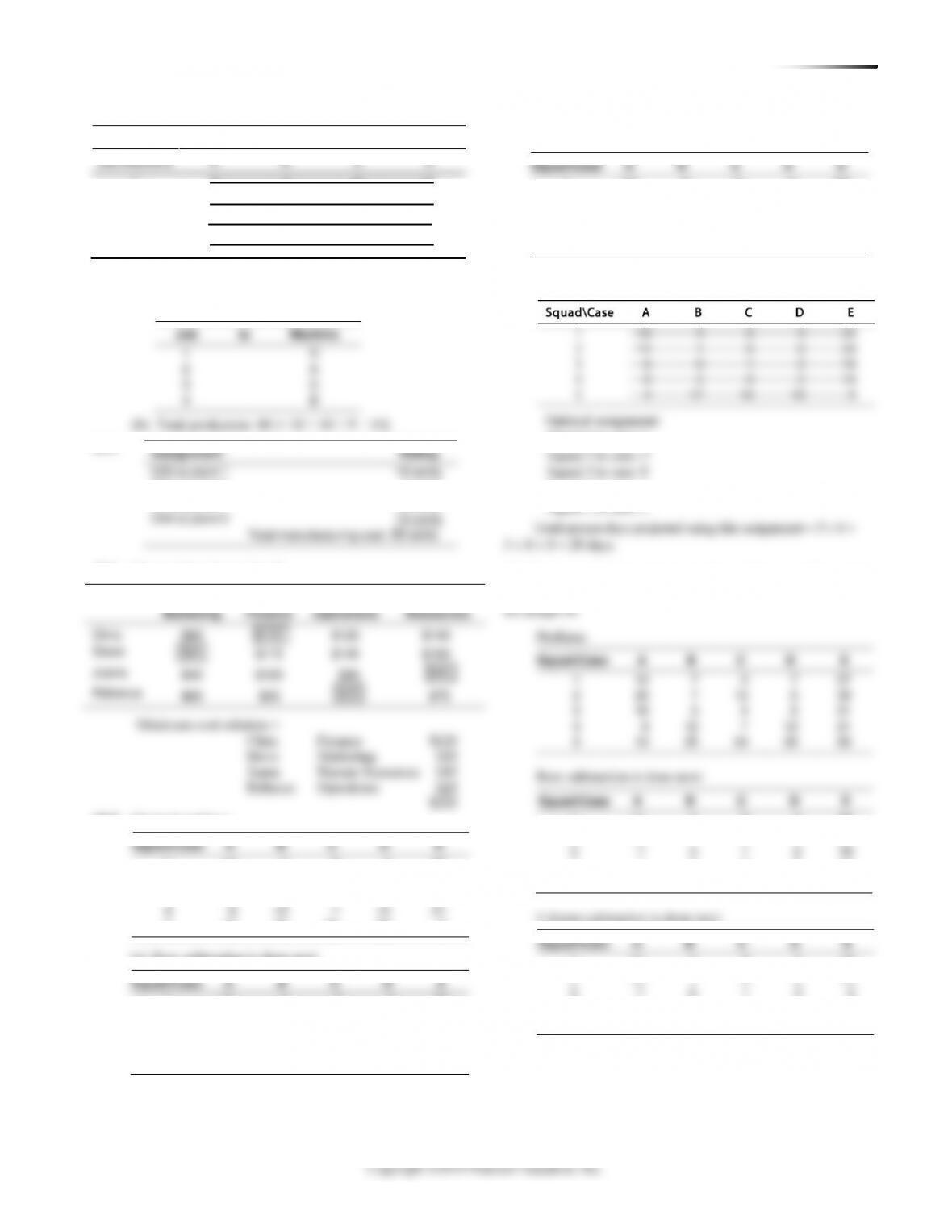
Squad\Case
A
B
C
D
1
7
3
7
2
20
7
12
6
3
10
3
4
5
4
8
12
7
12
5
13
25
26
1
11
4
0
4
24
2
14
1
6
0
24
3
7
0
1
2
18
4
1
5
0
5
14
5
5
17
16
0
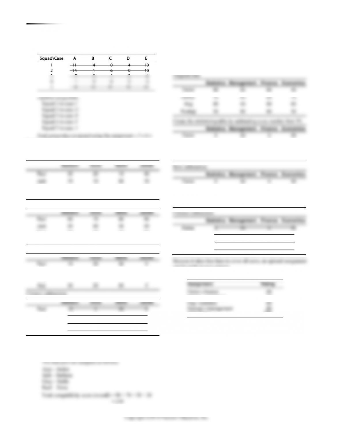
Squad\Case
A
B
C
D
E
11
4
0
4
24
14
1
6
0
24
7
0
1
2
18
1
5
0
5
14
0
12
11
13
37
Squad\Case
A
B
C
D
E
11
4
0
4
10
14
1
6
0
10
7
0
1
2
4
1
5
0
5
0
0
12
11
13
23
Squad\Case
A
B
C
D
1
7
3
7
2
20
7
12
6
3
10
3
4
5
4
8
12
7
12
5
13
25
26
1
11
4
0
4
24
2
14
1
6
0
24
3
7
0
1
2
18
4
1
5
0
5
14
5
5
17
16
0
Squad\Case
A
B
C
D
E
11
4
0
4
24
14
1
6
0
24
7
0
1
2
18
1
5
0
5
14
0
12
11
13
37
Squad\Case
A
B
C
D
E
11
4
0
4
10
14
1
6
0
10
7
0
1
2
4
1
5
0
5
0
0
12
11
13
23
Cover zeros with lines:
Squad 1 to case C
Squad 2 to case D
Squad 3 to case B
Squad 4 to case A
Squad 5 to case E
(b) We can avoid the assignment of squad 5 to case E occurring
by assigning a very high value to that combination. In this case,
we assign 50.
Problem:
Assignment
Rating
C53 at plant 1
10 cents
C81 at plant 3
4 cents
D5 at plant 4
30 cents
Column subtraction is done next:
Squad\Case
A
B
C
D
E
1
10
4
0
4
24
2
13
1
6
0
24
3
6
0
1
2
18
4
0
5
0
5
14
5
4
17
16
18
0
242 CHAPTER 15 SH O R T –T E R M SC H E D U L I N G
Cover zeros with lines:
Golhar
70
60
80
75
Hug
40
60
Create the minimizing table by subtracting every number from 95:
Statistics
Management
Finance
Economics
Fisher
5
30
0
55
Golhar
70
60
80
75
Hug
40
60
Create the minimizing table by subtracting every number from 95:
Statistics
Management
Finance
Economics
Fisher
5
30
0
55
3 + 21 + 13 = 46.
15.8
Original data:
Barbara
Dona
Stella
Jackie
Raul
30
20
10
40
Jack
70
10
60
70
Gray
40
20
50
40
Ajay
60
70
30
90
Create the minimizing table by subtracting every number from 90:
Barbara
Dona
Stella
Jackie
Raul
60
70
80
50
Jack
20
80
30
20
Gray
50
70
40
50
Ajay
30
20
60
0
Row subtraction:
Barbara
Dona
Stella
Jackie
Raul
10
20
30
0
Jack
0
60
10
0
Gray
10
30
0
10
Ajay
30
20
60
0
Column subtraction:
Barbara
Dona
Stella
Jackie
Raul
10
0
30
0
Jack
0
40
10
0
Gray
10
10
0
10
Ajay
0
0
Ajay
30
20
60
0
Column subtraction:
Barbara
Dona
Stella
Jackie
Raul
10
0
30
0
Jack
0
40
10
0
Gray
10
10
0
10
Ajay
0
0
15.9 Because this is a maximization problem, each number is
subtracted from 95. The problem is then solved using the
minimization algorithm.
(a)
Statistics
Management
Finance
Economics
Fisher
90
65
95
40
Golhar
25
35
15
20
Hug
10
55
15
35
Rustagi
40
15
30
40
Row subtraction:
Statistics
Management
Finance
Economics
Fisher
5
30
0
55
Golhar
10
20
0
5
Hug
0
45
5
25
Rustagi
25
0
15
25
Column subtraction:
Statistics
Management
Finance
Economics
Fisher
5
30
0
50
Golhar
10
20
0
0
Hug
0
45
5
20
Rustagi
25
0
15
20
Because it takes four lines to cover all zeros, an optimal assignment
can be made at zero squares.
CHAPTER 15 SH O R T –T E R M SC H E D U L I N G 243
Due Date
E
314
7
5
D
314
5
E
314
3
Due Date
E
314
7
5
D
314
5
E
314
3
Job Sequence
Due Date
B
312
A
313
D
314
Job
Due Date
Duration (Days)
A
313
8
B
312
16
C
325
40
244 CHAPTER 15 SH O R T –T E R M SC H E D U L I N G
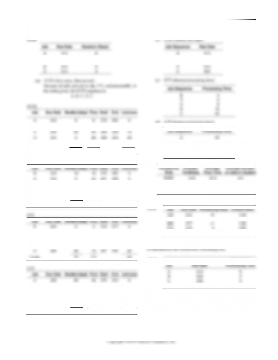
(a) First come, first served (FCFS):
Job
Processing
Time
Due
Date
Start
End
Days Late
A
6
212
205
210
0
B
3
209
211
213
4
C
3
208
214
216
8
D
8
210
217
224
14
Total: 26 days
Job
Processing
Time
Due
Date
Start
End
Days Late
B
3
209
205
207
0
C
3
208
208
210
2
A
6
212
211
216
4
D
8
210
217
224
14
Total: 20 days
LPT
9.0
14.8
3.0
LPT
9.0
14.8
3.0
Job
Processing
Time
Due
Date
Start
End
Days Late
D
8
210
205
212
2
A
6
212
213
218
6
C
3
208
219
221
13
B
3
209
222
224
15
Total: 36 days
(d) Earliest due date (EDD):
Job
Processing
Time
Due
Date
Start
End
Days Late
C
3
208
205
207
0
B
3
209
208
210
1
D
8
210
211
218
8
A
6
212
219
224
12
Total: 21 days
A
212
B
209
C
208
8
(210 – 205)/8 = 0.63
1.33
A
212
B
209
C
208
8
(210 – 205)/8 = 0.63
1.33
Critical ratio:
Job
Processing
Time
Due
Date
Start
End
Days Late
D
8
210
205
212
2
C
3
208
213
215
7
A
6
212
216
221
9
B
3
209
222
224
15
Total: 33
days
A minimum total lateness of 20 days seems to be about the
least we may achieve.
Average
Number
Scheduling
Average
Average
of Jobs in
Rule
Lateness
Flow Time
System
FCFS
6.5
11.8
2.4
SPT
5.0
10.25
2.1
EDD
5.25
10.8
2.2
Critical ratio
8.3
14.0
2.8
SPT is best on all criteria.

CHAPTER 15 SH O R T –T E R M SC H E D U L I N G 245
15.13 (a)
Dispatching
Rule
Job Sequence
Flow Time
Utilization
Average Number
of Jobs
Average Late
EDD
CX–BR–SY–DE–RG
385
37.6%
2.66
10
SPT
BR–CX–SY–DE–RG
375
38.6%
2.59
12
LPT
RG–DE–SY–CX–BR
495
29.3%
3.41
44
FCFS
CX–BR–DE–SY–RG
390
37.2%
2.69
12
Starting day number: 241 (i.e., work can be done on day 241)
Method: SPT—Shortest processing time
Processing
Time
Due Date
Order
Flow Time
Completion
Time
Late
CX–01
25
270
2
40
280
10
BR–02
15
300
1
15
255
0
DE–06
35
320
4
105
345
25
SY–11
30
310
3
70
310
0
RG–05
40
360
5
145
385
25
Total
145
375
60
Average
75
12
Sequence: BR-02,CX-01,SY-11,DE-06,RG-05, Average # in system = 2.586 = 375/145
Method: LPT—Longest processing time
Processing
Time
Due Date
Order
Flow Time
Completion
Time
Late
CX–01
25
270
4
130
370
100
BR–02
15
300
5
145
385
85
DE–06
35
320
2
75
315
0
SY–11
30
310
3
105
345
35
RG–05
40
360
1
40
280
0
Total
145
495
220
Average
99
44
Sequence: RG-05,DE-06,SY-11,CX-01,BR-02, Average # in system = 3.414 = 495/145
Method: Earliest due date (EDD); earliest to latest date
Processing Time
Due Date
Slack
Order
Flow Time
Completion Time
Late
CX–01
25
270
0
1
25
265
0
BR–02
15
300
0
2
40
280
0
DE–06
35
320
0
4
105
345
25
SY–11
30
310
0
3
70
310
0
RG–05
40
360
0
5
145
385
25
Total
145
385
50
Average
77
10
Sequence: CX-01,BR-02,SY-11,DE-06,RG-05, Average # in system = 2.655 = 385/145
Method: First come, first served (FCFS)
Processing Time
Due Date
Slack
Order
Flow Time
Completion Time
Late
CX–01
25
270
0
1
25
265
0
BR–02
15
300
0
2
40
280
0
DE–06
35
320
0
3
75
315
0
SY–11
30
310
0
4
105
345
35
RG–05
40
360
0
5
145
385
25
Total
145
390
60
Average
78
12
Sequence: CX-01,BR-02,DE-06,SY-11,RG-05, Average # in system = 2.69 = 390/145
246 CHAPTER 15 SH O R T –T E R M SC H E D U L I N G
(b) The best flow time is SPT; (c) best utilization is SPT;
B
30
B
30
15.14
10
16
18
20
Date
Critical
10
16
18
20
Date
Critical
(d) LPT (longest processing time):
A
20
E
18
D
16
C
10
Average
Number
Scheduling
Average
Average
of Jobs in
Job
Date
Order
Received
Production
Days
Needed
Date
Order
Due
A
110
20
180
B
120
30
200
C
122
10
175
D
125
16
230
240 CHAPTER 15 SH O R T –T E R M SC H E D U L I N G
2. Use the scrollbar to change the processing time for job C and
use the scrollbar to modify the due date for job C. Does the same
rule always minimize the average completion time?
3. Which schedule (rule) minimizes the average lateness for this
15.2
15.3 Original problem:
15.4 (a)
Original data
1
7
8
8
10
2
10
9
7
6
3
11
5
9
6
4
9
11
5
8
First, we create a minimizing table by subtracting every number from 11
Job/Machine
A
B
C
D
1
4
2
3
1
2
1
2
4
5
3
0
6
2
5
4
2
0
6
3
then we do row subtraction:
Job/Machine
A
B
C
D
1
3
1
2
0
2
0
1
3
4
3
0
6
2
5
4
2
0
6
3
Site/Customer
A
B
C
D
4
8
6
7
4
CHAPTER 15 SH O R T –T E R M SC H E D U L I N G 241
then we do column subtraction:
Job/Machine
A
B
C
D
1
3
1
0
0
2
0
1
1
4
3
0
6
0
5
4
2
0
4
3
Because it takes four lines to cover all zeros, an optimal
assignment can be made at zero squares.
Assignment:
15.5
15.6 Convert the minutes into $:
Marketing
Finance
Operations
Human
Resources
Chris
$80
$120
$125
$140
Cover zeros with lines:
Squad 1 to case C
Squad 2 to case D
Squad 3 to case B
Squad 4 to case A
Squad 5 to case E
(b) We can avoid the assignment of squad 5 to case E occurring
by assigning a very high value to that combination. In this case,
we assign 50.
Problem:
Assignment
Rating
C53 at plant 1
10 cents
C81 at plant 3
4 cents
D5 at plant 4
30 cents
Column subtraction is done next:
Squad\Case
A
B
C
D
E
1
10
4
0
4
24
2
13
1
6
0
24
3
6
0
1
2
18
4
0
5
0
5
14
5
4
17
16
18
0
242 CHAPTER 15 SH O R T –T E R M SC H E D U L I N G
Cover zeros with lines:
3 + 21 + 13 = 46.
15.8
Original data:
Barbara
Dona
Stella
Jackie
Raul
30
20
10
40
Jack
70
10
60
70
Gray
40
20
50
40
Ajay
60
70
30
90
Create the minimizing table by subtracting every number from 90:
Barbara
Dona
Stella
Jackie
Raul
60
70
80
50
Jack
20
80
30
20
Gray
50
70
40
50
Ajay
30
20
60
0
Row subtraction:
Barbara
Dona
Stella
Jackie
Raul
10
20
30
0
Jack
0
60
10
0
Gray
10
30
0
10
15.9 Because this is a maximization problem, each number is
subtracted from 95. The problem is then solved using the
minimization algorithm.
(a)
Statistics
Management
Finance
Economics
Fisher
90
65
95
40
Golhar
25
35
15
20
Hug
10
55
15
35
Rustagi
40
15
30
40
Row subtraction:
Statistics
Management
Finance
Economics
Fisher
5
30
0
55
Golhar
10
20
0
5
Hug
0
45
5
25
Rustagi
25
0
15
25
Column subtraction:
Statistics
Management
Finance
Economics
Fisher
5
30
0
50
Golhar
10
20
0
0
Hug
0
45
5
20
Rustagi
25
0
15
20
Because it takes four lines to cover all zeros, an optimal assignment
can be made at zero squares.
CHAPTER 15 SH O R T –T E R M SC H E D U L I N G 243
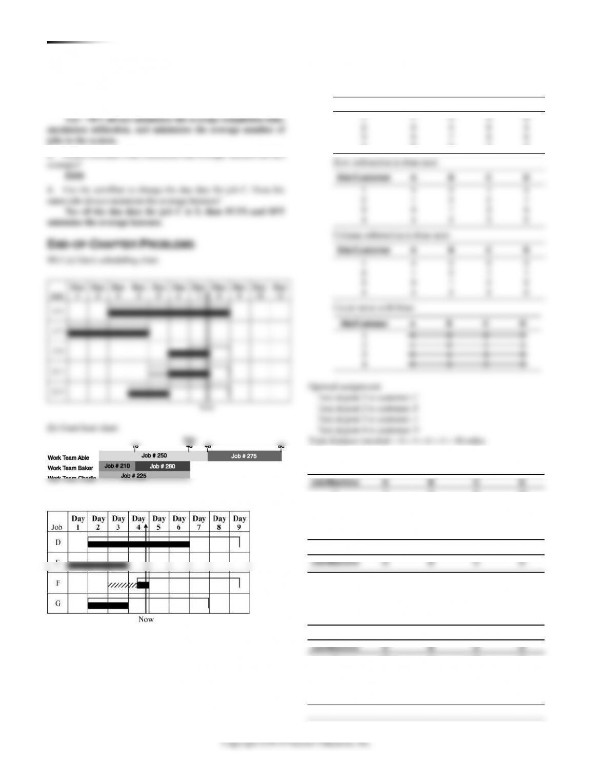
Job Sequence
Due Date
B
312
A
313
D
314
Job
Due Date
Duration (Days)
A
313
8
B
312
16
C
325
40
244 CHAPTER 15 SH O R T –T E R M SC H E D U L I N G
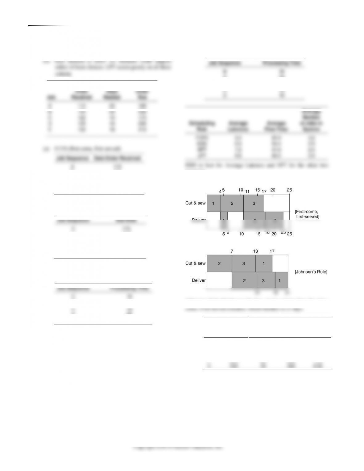
(a) First come, first served (FCFS):
Job
Processing
Time
Due
Date
Start
End
Days Late
A
6
212
205
210
0
B
3
209
211
213
4
C
3
208
214
216
8
D
8
210
217
224
14
Total: 26 days
Job
Processing
Time
Due
Date
Start
End
Days Late
B
3
209
205
207
0
C
3
208
208
210
2
A
6
212
211
216
4
D
8
210
217
224
14
Total: 20 days
Job
Processing
Time
Due
Date
Start
End
Days Late
D
8
210
205
212
2
A
6
212
213
218
6
C
3
208
219
221
13
B
3
209
222
224
15
Total: 36 days
(d) Earliest due date (EDD):
Job
Processing
Time
Due
Date
Start
End
Days Late
C
3
208
205
207
0
B
3
209
208
210
1
D
8
210
211
218
8
A
6
212
219
224
12
Total: 21 days
Critical ratio:
Job
Processing
Time
Due
Date
Start
End
Days Late
D
8
210
205
212
2
C
3
208
213
215
7
A
6
212
216
221
9
B
3
209
222
224
15
Total: 33
days
A minimum total lateness of 20 days seems to be about the
least we may achieve.
Average
Number
Scheduling
Average
Average
of Jobs in
Rule
Lateness
Flow Time
System
FCFS
6.5
11.8
2.4
SPT
5.0
10.25
2.1
EDD
5.25
10.8
2.2
Critical ratio
8.3
14.0
2.8
SPT is best on all criteria.
CHAPTER 15 SH O R T –T E R M SC H E D U L I N G 245
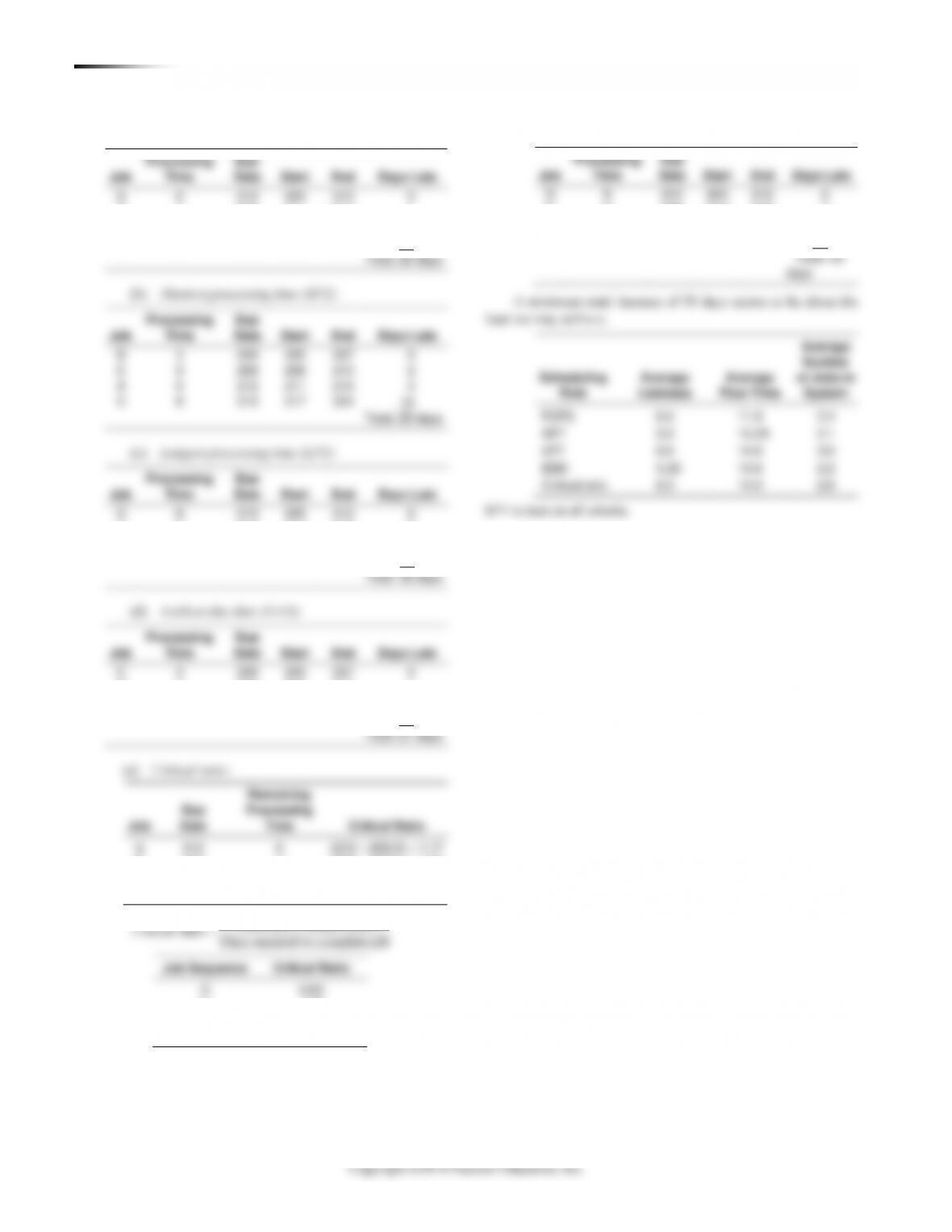
15.13 (a)
Dispatching
Rule
Job Sequence
Flow Time
Utilization
Average Number
of Jobs
Average Late
EDD
CX–BR–SY–DE–RG
385
37.6%
2.66
10
SPT
BR–CX–SY–DE–RG
375
38.6%
2.59
12
LPT
RG–DE–SY–CX–BR
495
29.3%
3.41
44
FCFS
CX–BR–DE–SY–RG
390
37.2%
2.69
12
Starting day number: 241 (i.e., work can be done on day 241)
Method: SPT—Shortest processing time
Processing
Time
Due Date
Order
Flow Time
Completion
Time
Late
CX–01
25
270
2
40
280
10
BR–02
15
300
1
15
255
0
DE–06
35
320
4
105
345
25
SY–11
30
310
3
70
310
0
RG–05
40
360
5
145
385
25
Total
145
375
60
Average
75
12
Sequence: BR-02,CX-01,SY-11,DE-06,RG-05, Average # in system = 2.586 = 375/145
Method: LPT—Longest processing time
Processing
Time
Due Date
Order
Flow Time
Completion
Time
Late
CX–01
25
270
4
130
370
100
BR–02
15
300
5
145
385
85
DE–06
35
320
2
75
315
0
SY–11
30
310
3
105
345
35
RG–05
40
360
1
40
280
0
Total
145
495
220
Average
99
44
Sequence: RG-05,DE-06,SY-11,CX-01,BR-02, Average # in system = 3.414 = 495/145
Method: Earliest due date (EDD); earliest to latest date
Processing Time
Due Date
Slack
Order
Flow Time
Completion Time
Late
CX–01
25
270
0
1
25
265
0
BR–02
15
300
0
2
40
280
0
DE–06
35
320
0
4
105
345
25
SY–11
30
310
0
3
70
310
0
RG–05
40
360
0
5
145
385
25
Total
145
385
50
Average
77
10
Sequence: CX-01,BR-02,SY-11,DE-06,RG-05, Average # in system = 2.655 = 385/145
Method: First come, first served (FCFS)
Processing Time
Due Date
Slack
Order
Flow Time
Completion Time
Late
CX–01
25
270
0
1
25
265
0
BR–02
15
300
0
2
40
280
0
DE–06
35
320
0
3
75
315
0
SY–11
30
310
0
4
105
345
35
RG–05
40
360
0
5
145
385
25
Total
145
390
60
Average
78
12
Sequence: CX-01,BR-02,DE-06,SY-11,RG-05, Average # in system = 2.69 = 390/145
246 CHAPTER 15 SH O R T –T E R M SC H E D U L I N G
(b) The best flow time is SPT; (c) best utilization is SPT;
15.14
(d) LPT (longest processing time):
A
20
E
18
D
16
C
10
Average
Number
Scheduling
Average
Average
of Jobs in
Job
Date
Order
Received
Production
Days
Needed
Date
Order
Due
A
110
20
180
B
120
30
200
C
122
10
175
D
125
16
230