
12
C H A P T E R
Inventory Management
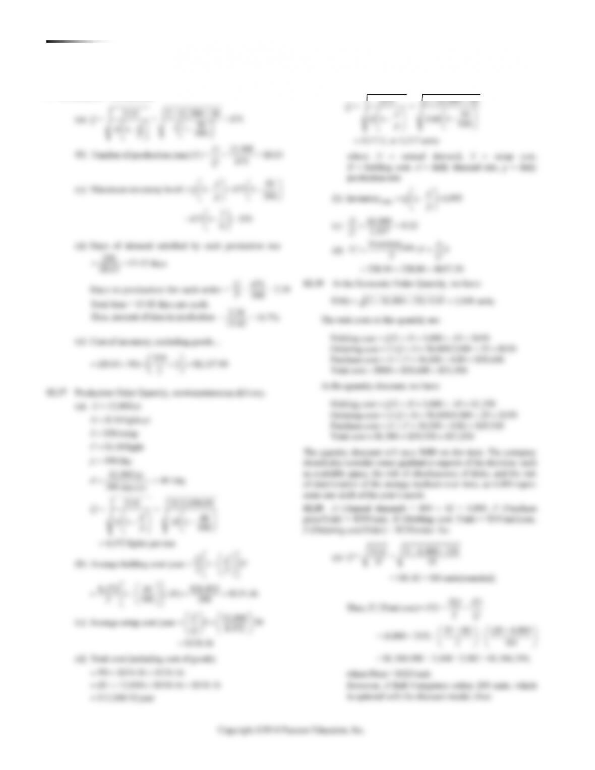
1. The four types of inventory are:
Raw material—items that are to be converted into product
◼ Work-in-process (WIP)—items that are in the process of
being converted
2. The advent of low-cost computing should not be seen as
obviating the need for the ABC inventory classification scheme.
Although the cost of computing has decreased considerably, the
3. The purpose of the ABC system is to identify those items that
require more attention due to cost or volume.
4. Types of costs—holding cost: the cost of capital invested and
space required; shortage cost: the cost of lost sales or customers
who never return; the cost of lost good will; ordering cost: the
ble costs are the costs of placing an order or setting up production
6. The EOQ increases as demand increases or as the setup cost
increases; it decreases as the holding cost increases. The changes
7. Price times quantity is not variable in the EOQ model but
is variable in the discount model. When quality discounts are
available, the unit purchase price of the item depends on the order
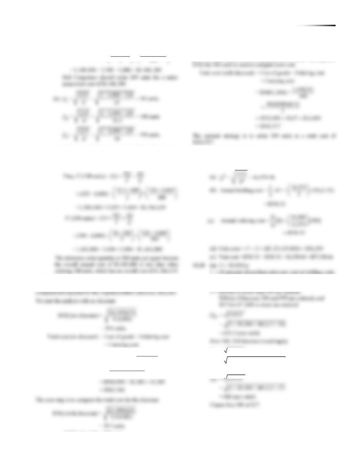
necessary for annual physical inventories
2. Eliminating annual inventory adjustments
3. Providing trained personnel to audit the accuracy of
inventory
4. Allowing the cause of errors to be identified and remedial
and the prices are no lower than at the EOQ. Points above the EOQ
have higher inventory costs than the corresponding price break
point or EOQ at prices that are no lower than either of the price
product or service is delivered when and as promised.
12. If the same costs hold, more will be ordered using the pro-
duction order quantity model because the average inventory is less
than the corresponding EOQ system.
13. In a fixed-quantity inventory system, when the quantity on
hand reaches the reorder point, an order is placed for the specified
14. The EOQ model gives quite good results under inexact inputs;
lead time, held to control the level of shortages when demand
and/or lead time are not constant; inventory carried to assure that
16. The reorder point is a function of: demand per unit of time,
lead time, customer service level, and standard deviation of demand.
17. Most retail stores have a computerized cash register (point–
172 CHAPTER 12 INV E N T O R Y MA N A G E M E N T
18. Advantage of a fixed period system: There is no physical
There is a possibility of stockout during the time between
orders.
1. What is the EOQ, and what is the lowest total cost?
EOQ = 200 units with a cost of $100
2. What is the annual cost of carrying inventory at the EOQ
and the annual cost of ordering inventory at the EOQ of
200 units?
$50 for carrying and also $50 for ordering
3. From the graph, what can you conclude about the relationship
between the lowest total cost and the costs of ordering and carry-
ing inventory?
4. How much does the total cost increase if the store manager
orders 50 more hypodermics than the EOQ? 50 fewer hypodermics?
Ordering more increases costs by $2.50, or 2.5%. Ordering
5. What happens to the EOQ and total cost when demand is
doubled? When carrying cost is doubled?
The EOQ rises by 82 units (41%) and the total cost rises
Copyright ©2014 Pearson Education, Inc.
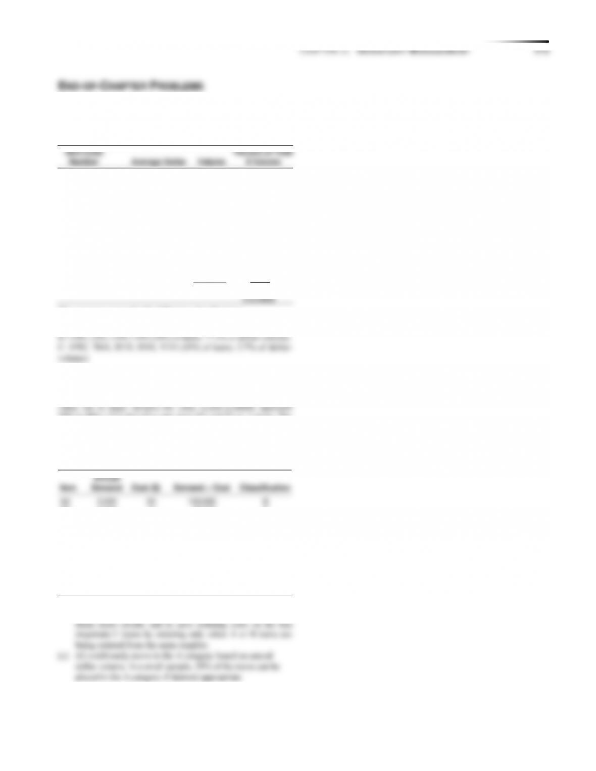
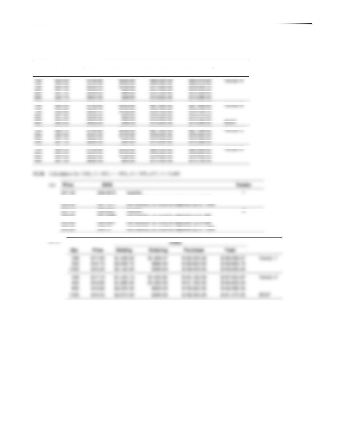
12.1 An ABC system generally classifies the top 70% of dollar
volume items as A, the next 20% as B, and the remaining 10% as
C items. Similarly, A items generally constitute 20% of total
number of items, B items are 30%; and C items are 50%.
Item Code
Number
Average Dollar
Volume
Percent of Total
$ Volume
1289
→
400 3.75 =
1,500.00
44.0%
2347
→
300 4.00 =
1,200.00
36.0%
2349
→
120 2.50 =
300.00
9.0%
2363
→
75 1.50 =
112.50
3.3%
2394
→
60 1.75 =
105.00
3.1%
2395
→
30 2.00 =
60.00
1.8%
6782
→
20 1.15 =
23.00
0.7%
7844
→
12 2.05 =
24.60
0.7%
8210
→
8 1.80 =
14.40
0.4%
8310
→
7 2.00 =
14.00
0.4%
9111
→
6 3.00 =
18.00
0.5%
$3,371.50
100%
(rounded)
The company can make the following classifications:
A: 1289, 2347 (18% of items; 80% of dollar-volume).
12.2 (a) You decide that the top 20% of the 10 items, based on a
criterion of demand times cost per unit, should be A items. (In this
example, the top 20% constitutes only 58% of the total inventory
70% to 80%.) You therefore rate items F3 and G2 as A items. The
next 30% of the items are A2, C7, and D1; they represent 23% of
the value and are categorized as B items. The remaining 50% of
the items (items B8, E9, H2, I5, and J8) represent 19% of the
value and become C items.
Annual
Item
Demand
Cost ($)
Demand Cost
Classification
A2
3,000
50
150,000
B
B8
4,000
12
48,000
C
C7
1,500
45
67,500
B
D1
6,000
10
60,000
B
E9
1,000
20
20,000
C
F3
500
500
250,000
A
G2
300
1,500
450,000
A
H2
600
20
12,000
C
I5
1,750
10
17,500
C
J8
2,500
5
12,500
C
(b) Borecki can use this information to manage his A and B
174 CHAPTER 12 INV E N T O R Y MA N A G E M E N T
12.3
Inventory
Item
$Value
per
Case
#Ordered
per
Week
Total $
Value/Week
(52 Weeks)
Total = ($*52)
Rank
Percent of
Inventory
Cumulative
Percent of
Inventory
Fish filets
143
10
$1,430
$74,360
1
17.54%
17.54%
French fries
43
32
$1,376
$71,552
2
16.88%
34.43%
Chickens
75
14
$1,050
$54,600
3
12.88%
47.31%
Prime rib
166
6
$996
$51,792
4
12.22%
59.53%
Lettuce (case)
35
24
$840
$43,680
5
10.31%
69.83%
Lobster tail
245
3
$735
$38,220
6
9.02%
78.85%
Rib eye steak
135
3
$405
$21,060
7
4.97%
83.82%
Bacon
56
5
$280
$14,560
8
3.44%
87.25%
Pasta
23
12
$276
$14,352
9
3.39%
90.64%
Tomato sauce
23
11
$253
$13,156
10
3.10%
93.74%
Tablecloths
32
5
$160
$8,320
11
1.96%
95.71%
Eggs (case)
22
7
$154
$8,008
12
1.89%
97.60%
Oil
28
2
$56
$2,912
13
0.69%
98.28%
Trashcan liners
12
3
$36
$1,872
14
0.44%
98.72%
Garlic powder
11
3
$33
$1,716
15
0.40%
99.13%
Napkins
12
2
$24
$1,248
16
0.29%
99.42%
Order pads
12
2
$24
$1,248
17
0.29%
99.72%
Pepper
3
3
$9
$468
18
0.11%
99.83%
Sugar
4
2
$8
$416
19
0.10%
99.93%
Salt
3
2
$6
$312
20
0.07%
100.00%
$8,151
$423,852
100.00%
(a) Fish filets total $74,360.
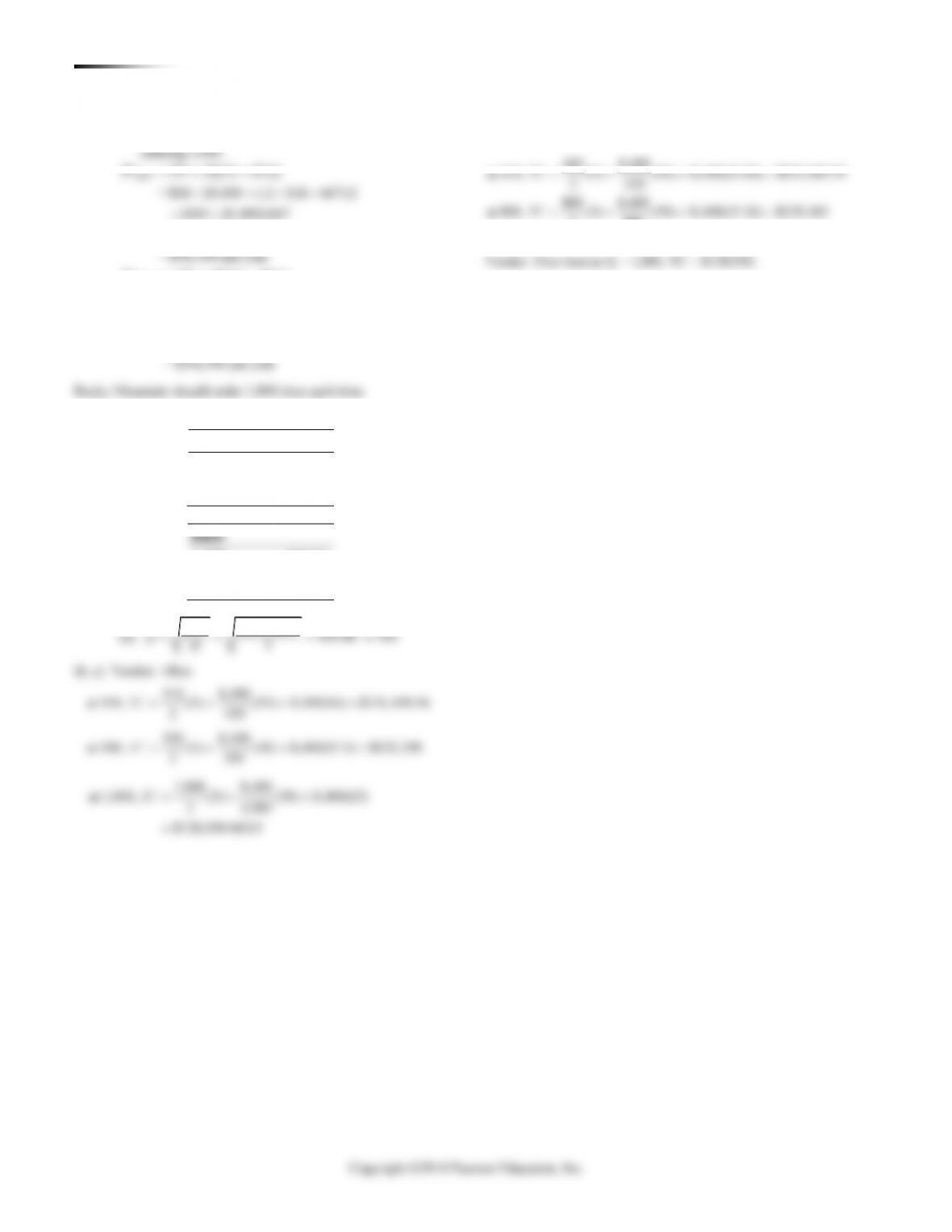
12.4
7,000 0.10 = 700
700 20 = 35
35 A items per day
7,000 0.35 = 2,450
2450 60 = 40.83
41 B items per day
7,000 0.55 = 3,850
3850 120 = 32
32 C items per day
108 items
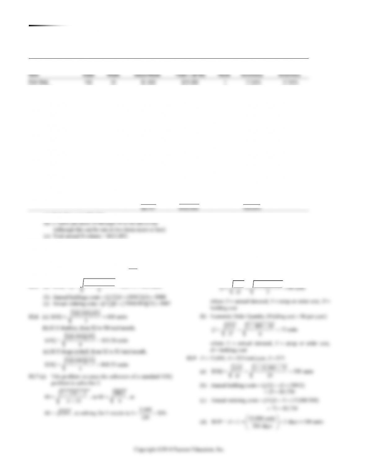
12.5 (a)
2(19,500)(25)
EOQ = 493.71 494 units
4
Q= = =
2(8,000)(45)
( )( )
2 8,000 45
(b) If S were $30, then the EOQ would be 60. If the true
ordering cost turns out to be much greater than $30,
then the firm’s order policy is ordering too little
at a time.
12.8 (a) Economic Order Quantity (Holding cost = $5 per year):
holding cost
6
2 2 400 40 80 units
5
DS
QH
= = =
176 CHAPTER 12 INV E N T O R Y MA N A G E M E N T
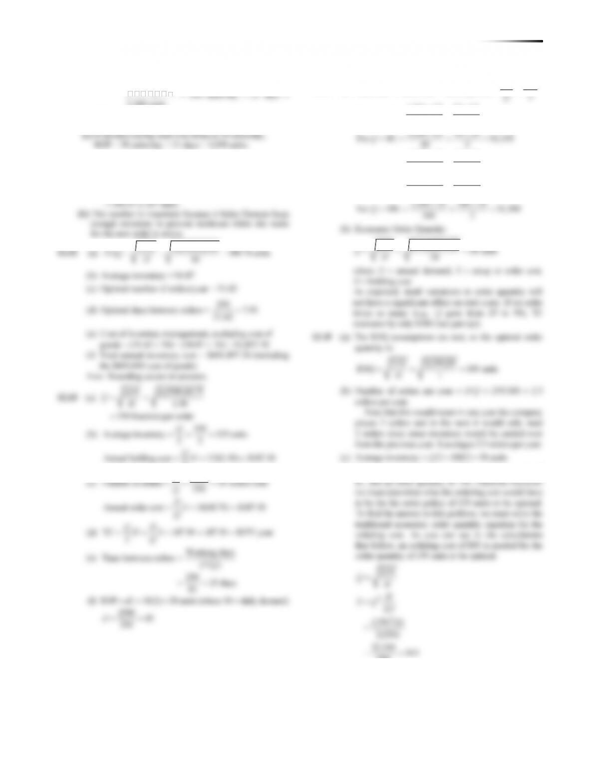
12.16 D = 12,500/year, so d = (12,500/250) = 50/day, p = 300/day,
S = $30/order, H = $2/unit/year
(a)
12.18 (a) Production Order Quantity, noninstantaneous delivery:
2 2 10,000 40
50
1
0.60
1500
DS
Q
d
Hp
==
−
−
DS
Qd
Hp
2 2 ×12,500 × 30
= = = 671
50
2 1 –
1– 300
181 units would not be bought at $350. 196 units can-
not be bought at $300, hence that isn’t possible either.
So, EOQ = 188 units.
$543,517.
12.22
= 45,000, = $200, = 5% of unit price, D S I H = IP
Best option must be determined first. Since all solutions yield Q
values greater than 10,000, the best option is the $1.25 price.
178 CHAPTER 12 INV E N T O R Y MA N A G E M E N T
(b) We compare the cost of ordering 667 with the cost of
667 /2 /
= $18 20,000 (.2 $18 667)/2
($40 20,000)/667
= $360,000 + $1,200 + $1,200
= $362,400 per year
TC PD HQ SD Q= + +
+
+
1,000 /2 /
= $17 20,000 (.2 $17 1,000)/2
($40 20,000) /1,000
= $340,000 + $1,700 + $800
= $342,500 per year
TC PD HQ SD Q= + +
+
+
Rocky Mountain should order 1,000 tires each time.
12.24 D = 700 12 = 8,400, H = 5, S = 50
Allen
1–499
$16.00
500–999
$15.50
1,000+
$15.00
Baker
1–399
$16.10
400–799
$15.60
800+
$15.10
(a)
Vendor: Baker
Vendor Allen best at Q = 1,000, TC = $128,920.
410 8,400
at 410, (5) (50) 8,400(15.60) $133,089.39
2 410
800 8,400
at 800, (5) (50) 8,400(15.10) $129,365
2 800
TC
TC
= + + =
= + + =
2 2(8,400)50 409.88 410
5
DS
QH
= = = →
172 CHAPTER 12 INV E N T O R Y MA N A G E M E N T
18. Advantage of a fixed period system: There is no physical
There is a possibility of stockout during the time between
orders.
1. What is the EOQ, and what is the lowest total cost?
EOQ = 200 units with a cost of $100
2. What is the annual cost of carrying inventory at the EOQ
and the annual cost of ordering inventory at the EOQ of
200 units?
$50 for carrying and also $50 for ordering
3. From the graph, what can you conclude about the relationship
between the lowest total cost and the costs of ordering and carry-
ing inventory?
4. How much does the total cost increase if the store manager
orders 50 more hypodermics than the EOQ? 50 fewer hypodermics?
Ordering more increases costs by $2.50, or 2.5%. Ordering
5. What happens to the EOQ and total cost when demand is
doubled? When carrying cost is doubled?
The EOQ rises by 82 units (41%) and the total cost rises
Copyright ©2014 Pearson Education, Inc.
12.1 An ABC system generally classifies the top 70% of dollar
volume items as A, the next 20% as B, and the remaining 10% as
C items. Similarly, A items generally constitute 20% of total
number of items, B items are 30%; and C items are 50%.
Item Code
Number
Average Dollar
Volume
Percent of Total
$ Volume
1289
→
400 3.75 =
1,500.00
44.0%
2347
→
300 4.00 =
1,200.00
36.0%
2349
→
120 2.50 =
300.00
9.0%
2363
→
75 1.50 =
112.50
3.3%
2394
→
60 1.75 =
105.00
3.1%
2395
→
30 2.00 =
60.00
1.8%
6782
→
20 1.15 =
23.00
0.7%
7844
→
12 2.05 =
24.60
0.7%
8210
→
8 1.80 =
14.40
0.4%
8310
→
7 2.00 =
14.00
0.4%
9111
→
6 3.00 =
18.00
0.5%
$3,371.50
100%
(rounded)
The company can make the following classifications:
A: 1289, 2347 (18% of items; 80% of dollar-volume).
12.2 (a) You decide that the top 20% of the 10 items, based on a
criterion of demand times cost per unit, should be A items. (In this
example, the top 20% constitutes only 58% of the total inventory
70% to 80%.) You therefore rate items F3 and G2 as A items. The
next 30% of the items are A2, C7, and D1; they represent 23% of
the value and are categorized as B items. The remaining 50% of
the items (items B8, E9, H2, I5, and J8) represent 19% of the
value and become C items.
Annual
Item
Demand
Cost ($)
Demand Cost
Classification
A2
3,000
50
150,000
B
B8
4,000
12
48,000
C
C7
1,500
45
67,500
B
D1
6,000
10
60,000
B
E9
1,000
20
20,000
C
F3
500
500
250,000
A
G2
300
1,500
450,000
A
H2
600
20
12,000
C
I5
1,750
10
17,500
C
J8
2,500
5
12,500
C
(b) Borecki can use this information to manage his A and B
174 CHAPTER 12 INV E N T O R Y MA N A G E M E N T
12.3
Inventory
Item
$Value
per
Case
#Ordered
per
Week
Total $
Value/Week
(52 Weeks)
Total = ($*52)
Rank
Percent of
Inventory
Cumulative
Percent of
Inventory
Fish filets
143
10
$1,430
$74,360
1
17.54%
17.54%
French fries
43
32
$1,376
$71,552
2
16.88%
34.43%
Chickens
75
14
$1,050
$54,600
3
12.88%
47.31%
Prime rib
166
6
$996
$51,792
4
12.22%
59.53%
Lettuce (case)
35
24
$840
$43,680
5
10.31%
69.83%
Lobster tail
245
3
$735
$38,220
6
9.02%
78.85%
Rib eye steak
135
3
$405
$21,060
7
4.97%
83.82%
Bacon
56
5
$280
$14,560
8
3.44%
87.25%
Pasta
23
12
$276
$14,352
9
3.39%
90.64%
Tomato sauce
23
11
$253
$13,156
10
3.10%
93.74%
Tablecloths
32
5
$160
$8,320
11
1.96%
95.71%
Eggs (case)
22
7
$154
$8,008
12
1.89%
97.60%
Oil
28
2
$56
$2,912
13
0.69%
98.28%
Trashcan liners
12
3
$36
$1,872
14
0.44%
98.72%
Garlic powder
11
3
$33
$1,716
15
0.40%
99.13%
Napkins
12
2
$24
$1,248
16
0.29%
99.42%
Order pads
12
2
$24
$1,248
17
0.29%
99.72%
Pepper
3
3
$9
$468
18
0.11%
99.83%
Sugar
4
2
$8
$416
19
0.10%
99.93%
Salt
3
2
$6
$312
20
0.07%
100.00%
$8,151
$423,852
100.00%
(a) Fish filets total $74,360.
12.4
7,000 0.10 = 700
700 20 = 35
35 A items per day
7,000 0.35 = 2,450
2450 60 = 40.83
41 B items per day
7,000 0.55 = 3,850
3850 120 = 32
32 C items per day
108 items
12.5 (a)
2(19,500)(25)
EOQ = 493.71 494 units
4
Q= = =
2(8,000)(45)
( )( )
2 8,000 45
(b) If S were $30, then the EOQ would be 60. If the true
ordering cost turns out to be much greater than $30,
then the firm’s order policy is ordering too little
at a time.
12.8 (a) Economic Order Quantity (Holding cost = $5 per year):
holding cost
6
2 2 400 40 80 units
5
DS
QH
= = =
176 CHAPTER 12 INV E N T O R Y MA N A G E M E N T
12.16 D = 12,500/year, so d = (12,500/250) = 50/day, p = 300/day,
S = $30/order, H = $2/unit/year
(a)
12.18 (a) Production Order Quantity, noninstantaneous delivery:
2 2 10,000 40
50
1
0.60
1500
DS
Q
d
Hp
==
−
−
DS
Qd
Hp
2 2 ×12,500 × 30
= = = 671
50
2 1 –
1– 300
181 units would not be bought at $350. 196 units can-
not be bought at $300, hence that isn’t possible either.
So, EOQ = 188 units.
$543,517.
12.22
= 45,000, = $200, = 5% of unit price, D S I H = IP
Best option must be determined first. Since all solutions yield Q
values greater than 10,000, the best option is the $1.25 price.
178 CHAPTER 12 INV E N T O R Y MA N A G E M E N T
(b) We compare the cost of ordering 667 with the cost of
667 /2 /
= $18 20,000 (.2 $18 667)/2
($40 20,000)/667
= $360,000 + $1,200 + $1,200
= $362,400 per year
TC PD HQ SD Q= + +
+
+
1,000 /2 /
= $17 20,000 (.2 $17 1,000)/2
($40 20,000) /1,000
= $340,000 + $1,700 + $800
= $342,500 per year
TC PD HQ SD Q= + +
+
+
Rocky Mountain should order 1,000 tires each time.
12.24 D = 700 12 = 8,400, H = 5, S = 50
Allen
1–499
$16.00
500–999
$15.50
1,000+
$15.00
Baker
1–399
$16.10
400–799
$15.60
800+
$15.10
(a)
Vendor: Baker
Vendor Allen best at Q = 1,000, TC = $128,920.
410 8,400
at 410, (5) (50) 8,400(15.60) $133,089.39
2 410
800 8,400
at 800, (5) (50) 8,400(15.10) $129,365
2 800
TC
TC
= + + =
= + + =
2 2(8,400)50 409.88 410
5
DS
QH
= = = →