978-0123745071 Chapter 3 Quali…cations and Extensions

subject Type Homework Help
subject Pages 6
subject Words 1326
subject Authors Vijay Krishna

Unlock document.

This document is partially blurred.
Unlock all pages and 1 million more documents.
Get Access
page-pf1
4 Qualifications and Extensions
Problem 4.1 (Risk-averse bidders) There are two bidders with private values which
are distributed independently according to the uniform distribution F(x) = xover
[0;1] :Both bidders are risk-averse and have utility functions u(z) = pz: Find sym-
metric equilibrium bidding strategies in a first-price auction.
Solution. This is a special case of Example 4.1 with a= 1=2and F(x) = x, so
(x) = 1
F(x)Zx
0
yf(y)dy =1
x2Zx
0
y2ydy =2
3x
Problem 4.2 (Increase in risk aversion) Consider an N-bidder first-price auction
where each bidder’s value is distributed according to F: All bidders are risk averse with
a utility function uthat satisfies u(0) = 0; u0>0; u00 <0:Show that if one changed
the utility function of all bidders from u(z)to (u(z)), where is an increasing and
concave function satisfying (0) = 0;then this would lead to a higher symmetric
equilibrium bidding strategy.
Solution. Let be the equilibrium bidding strategy for utility uwhile ^be the
equilibrium bidding strategy for (u). From equation (4.2), we have
0(x) = u(x(x))
^0(x) = (u(x^(x)))
Notice that is strictly concave and (0) = 0, for all y > 0,(y)=0(y)> y.
Using this fact, for x > 0we have
^0(x) = (u(x^(x)))
or equivalently
It is also easy to check that
^(0) = (0) (3)
Equations (2) and (3) imply that for all x > 0;
11
page-pf2
Problem 4.3 (Asymmetric first-price auction) Suppose that bidder 1’s value X1is
distributed according to F1(x) = 1
4(x1)2over [1;3] and bidder 2’s value is distrib-
uted according to F2(x) = exp 2
3x2over [0;3] :
a. Show that 1(x) = x1and 2(x) = 2
3xconstitute equilibrium bidding strate-
gies in a first-price auction.
b. Compare the expected revenues in a first- and second-price auction.
Solution. Part a. Given bidder 2’s strategy 2(x) = 2
3x, bidder 1 with valuation
xchooses bto maximize his expected payo¤
F21
The first-order condition is
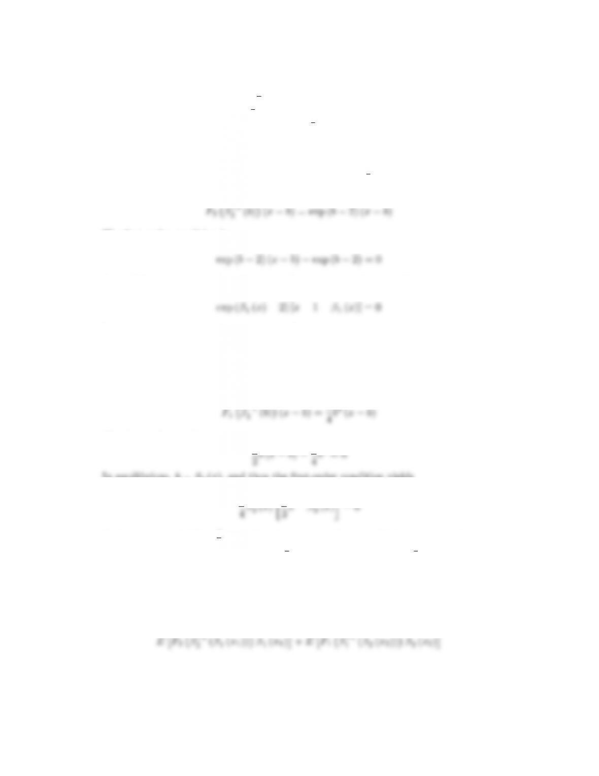
In equilibrium, b=1(x), and thus the first-order condition yields
It is easy to see that 1(x) = x1satisfies the equation above, and it is easy to see
that the marginal payo¤ is negative if 1(x)> x 1and positive if 1(x)< x 1;
therefore it is the best response to bid 1(x):
On the other hand, given bidder 1’s strategy 1(x) = x1, bidder 2 with
valuation xchooses bto maximize his expected payo¤
F11
4b2(xb)
The first-order condition is 1
In equilibrium, b=2(x), and thus the first-order condition yields
3
It obvious that 2(x) = 2
3xsatisfies the equation above, and it is easy to see that the
marginal payo¤ is negative if 2(x)>2
3xand positive if 2(x)<2
3x; therefore it is
the best response to bid 1(x):
In sum, given bidder 1’s strategy 1(x);bidder 2’s best response is 2(x), and
given bidder 2’s strategy 2(x)bidder 1’s best response is 1(x), therefore 1(x)
and 2(x)constitute an equilibrium.
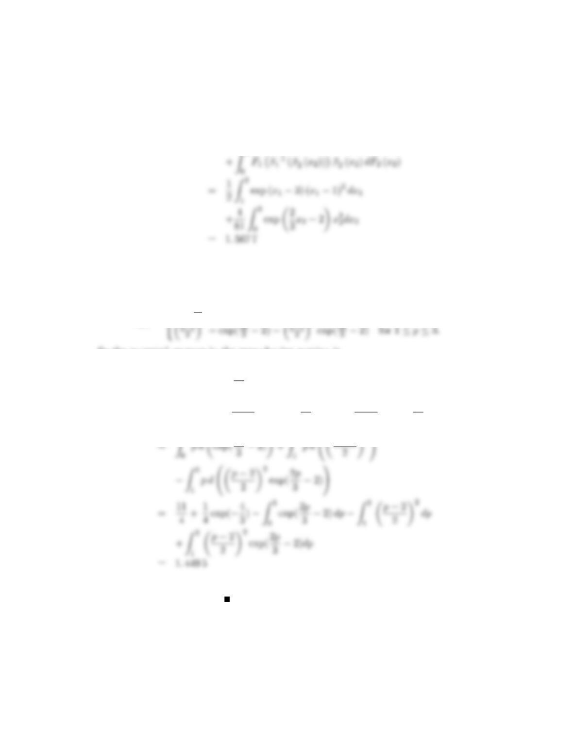
Part b. In the first-price auction, the expected revenue is
EF21
12
page-pf3
where the first term is the expected payment from bidder 1 and the second term is
the expected payment from bidder 2. Given the distributions and bidding strategies,
the expected revenue could be rewritten as
ERI=Z3
1
F21
2(1(x1))1(x1)dF1(x1)
In the second-price auction, it is a dominant strategy to bid one’s value. We
can either use the same method for the first price auction or calculate the expected
revenue using price distribution, and here we use the latter. The distribution of price
is
L(p) = 8
<
:
exp(2p
32) for p < 1
p2
So the expected revenue in the second-price auction is
ERII=Z1
0
p d exp(2p
32)
+Z3
1
p d p2
22
+ exp(2p
32) p2
22
exp(2p
32)!
=Z3
p d exp(2p
p d p2
where the third equality comes from integration by parts.
Thus, ERI> E RII.
Problem 4.4 (Equilibrium with reserve price) Suppose that bidder 1’s value X1is
distributed uniformly on [0;2] while bidder 2’s value X2is distributed uniformly on
13
page-pf4
[3
2;5
2]. The object is sold via a first-price auction with a reserve price r= 1. Verify
that 1(x) = x
2+1
2and 2(x) = x
2+1
4constitute equilibrium strategies.
Solution. F1(x) = x
2for x2[0;2] and F2(x) = x3
2for x23
2;5
2. Given bidder
2’s strategy 2(x) = x
2+1
4, bidder 1 with valuation xchooses bto maximize his
expected payo¤. If br, the expected payo¤ is
and the corresponding marginal payo¤ is
x2b+ 1
The first-order condition is
At equilibrium, b=1(x), and thus the first-order condition yields
It is easy to see that 1(x) = x+1
2satisfies the equation above. Moreover, it is easy to
see that the marginal payo¤ is negative if b > x+1
2and the marginal payo¤ is positive
if b < x+1
2:Therefore 1(x) = x+1
2is the best response to 2(x):
On the other hand, given bidder 1’s strategy 1(x) = x
2+1
2, bidder 2 with
valuation xchooses bto maximize his expected payo¤. If br, The expected payo¤
is
F11
1(b)(xb) = (2b1) (xb)=2
The first-order condition is
At equilibrium, b=2(x), and thus the first-order condition yields
It obvious that 2(x) = x
2+1
4satisfies the equation above, and it is bidder 2’s best
response to 1(x)by the same reasoning in the case of bidder 1.
We have shown that given bidder 1’s strategy 1(x)bidder 2’s best response
is 2(x), and given bidder 2’s strategy 2(x)bidder 1’s best response is 1(x).
Therefore 1and 2constitute an equilibrium.
Problem 4.5 (Discrete values) Suppose that there is no uncertainty about bidder 1’s
value and X1= 2 always. Bidder 2’s value, X2, is equally likely to be 0or 2.
a. Find equilibrium bidding strategies in a first-price auction. (Note that since
values are discrete, the equilibrium will be in mixed strategies.)
b. Compare the revenues in a first- and second-price auction.
14
page-pf5
Solution. Part a. Note that when bidder 2 has value 0, it is his weakly dominant
strategy to bid zero. Let us assume bidder 1’s mixed-strategy has cumulative dis-
tribution M1(b)and bidder 2 with valuation 2 has mixed-strategy with cumulative
distribution M2(b). We only consider the case that M1and M2are di¤erentiable.
If bidder 1 bid b, his expected payo¤ is
1
which is the product between the probability of winning and the payo¤ when he wins.
Because bidder 1 plays mixed-strategy, his expected payo¤ should be the same for
any bin the support of M1;therefore
1
where Cis a constant. So we have
M2(b) = 2C
2b1(4)
It should also be true that
M2(0) = 0 (5)
(4) and (5) imply that
If bidder 2 with valuation 2 bids b, this expected payo¤ is
M1(b) (2 b)
which is the product between the probability of winning and the payo¤ when he wins.
Similar to the analysis for bidder 1, we have
for some constant C0.
Because every bidder does not bid higher than his opponent, the highest bid is
the same for both bidders. Note that the highest bid for bidder 2 is 1, so we have
M1(1) = 1 (7)
(6) and (7) imply that
M1(b) = 1
where 0is a mass point of the distribution of M1:
15
page-pf6
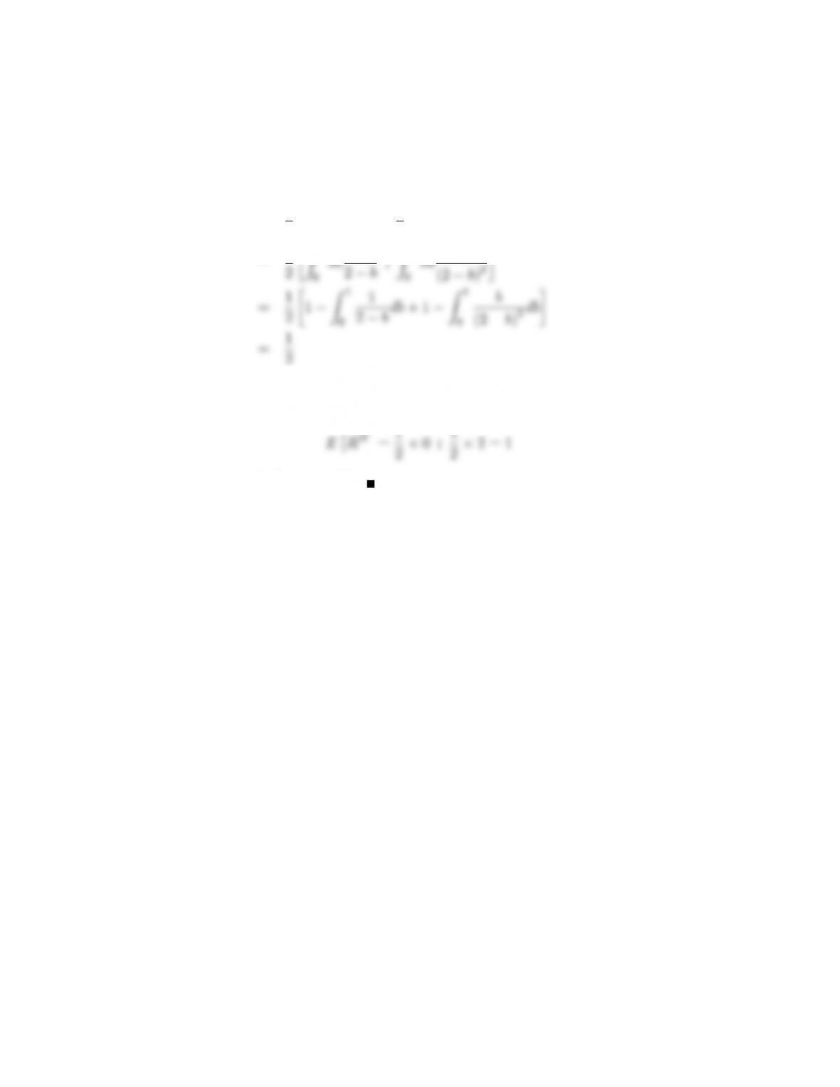
Part b. When X2= 0, the cumulative distribution for price is M1;and when
X2= 2, the cumulative distribution for price is M1M2, so the expected revenue in
the first-price auction is
ERI= Pr (X2= 0) E[PjX2= 0] + Pr (X2= 2) E[PjX2=]
=1
2Z1
0
bdM1(b) + 1
2Z1
0
bd [M1(b)M2(b)]
=1
bd 1
bd b
2
where the fourth equality comes from integration by parts.
The expected revenue in the second-price auction is
So we have ERI< E RII:
16

Trusted by Thousands of
Students

Here are what students say about us.

Copyright ©2022 All rights reserved. | CoursePaper is not sponsored or endorsed by any college or university.