Unlock document.
This document is partially blurred.
Unlock all pages and 1 million more documents.
Get Access
Chapter 7
Solution 7.1
Cost can be estimated using historic data correlations given in Table 7.1.
Solution 7.2
N = 6
Solution 7.3
See Example 7.5
forecast).
Solution 7.4
See solution to problem 7.3. With a longer extrapolation in time it is necessary to develop some sort of trend model
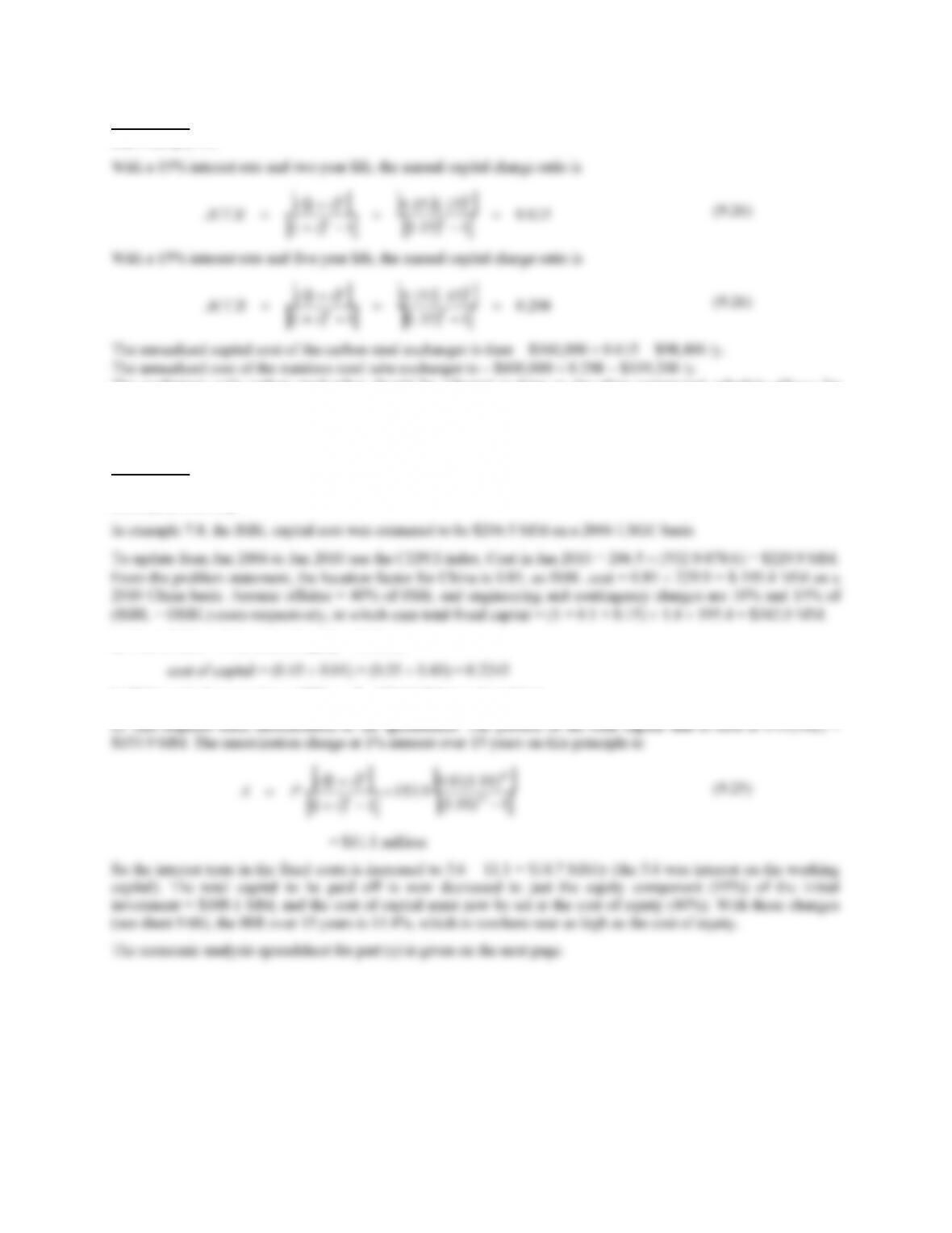
= 225000 × ⎟
⎠
⎜
⎝
5.389
Notes:
41
Solution 7.5
See Section 7.5. Cost equipment using Table 7.2 or using commercial costing software such as Aspen ICARUS.
We need to estimate the wall thickness to determine the shell mass (see example 7.3). The design pressure
should be 10% above the operating pressure (see Chapter 14), so the design pressure is 11 bar or roughly
12.9 ksi or roughly 89 N/mm2 (Table 14.2). Assuming the welds will be fully radiographed the weld
We can now calculate the shell mass, using the density of carbon steel (= 7900 kg/m3, from Table 6.2).
Shell mass =
π
Dc Lc tw
ρ
where: Dc = vessel diameter, m
basis.
42
For a vertical CS vessel, Table 7.2 gives:
Shell mass =
π
Dc Lc tw
ρ
where: Dc = vessel diameter, m
Lc = vessel length, m
Solution 7.6
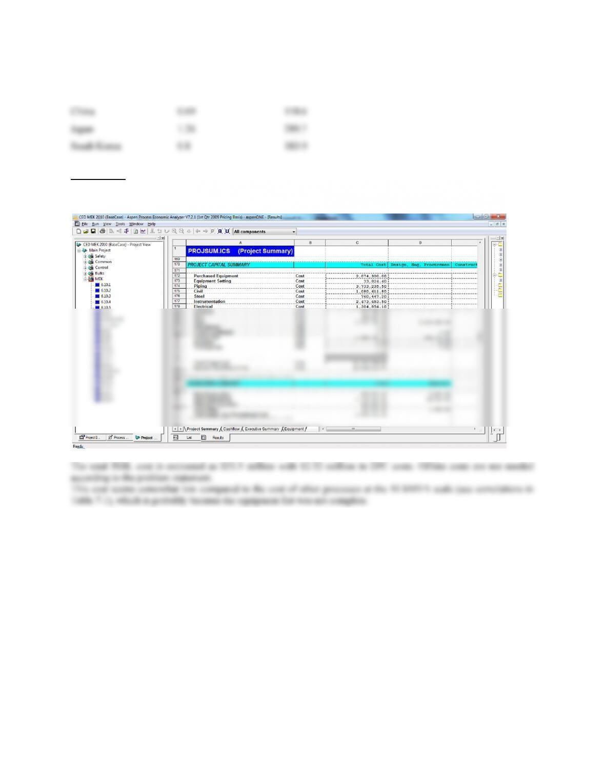
Using Aspen ICARUS, on a Jan 2010 basis:
Solution 7.7
a) From Aspen ICARUS equipment cost (not installed cost) on Jan 2010 USGC basis = $283,200
43
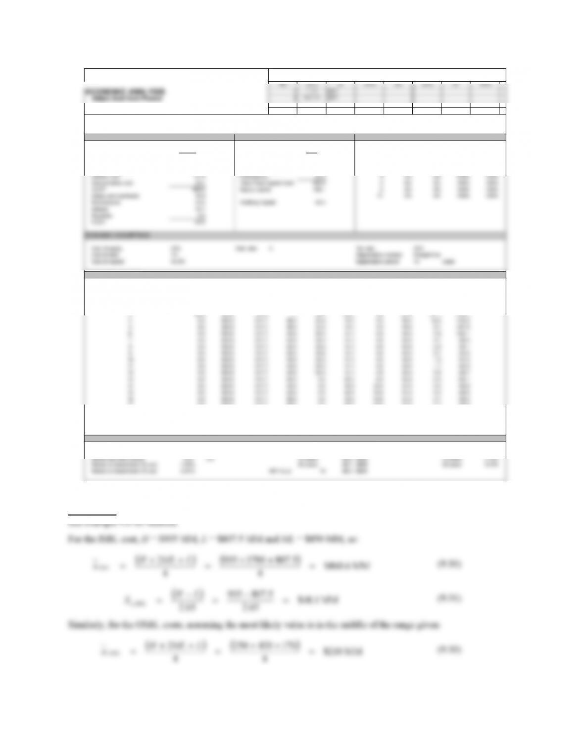
Solution 7.8
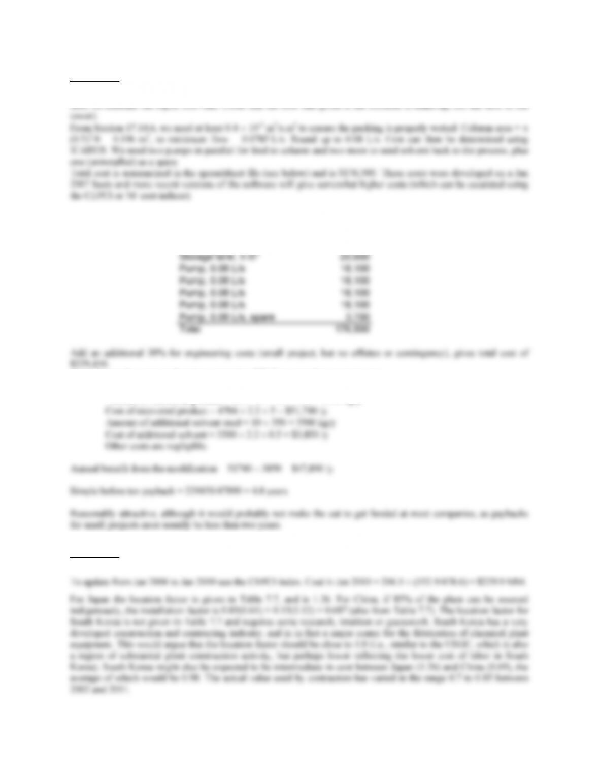
The tower and tank costs can be estimated using the information provided. The pump costs cannot be determined
until we estimate the liquid flow rate. (Note that the flow rate given is the increase in make-up, not the flow to the
Installed capital costs (from Aspen ICARUS)
k$
Tower + packing, 0.5 x 4 m 74,800
3
Annual operating costs and savings, assuming 350 days operation per year, are:
Amount of recovered product = 0.8 × 0.7 × 24 × 350 = 4704 kg/y
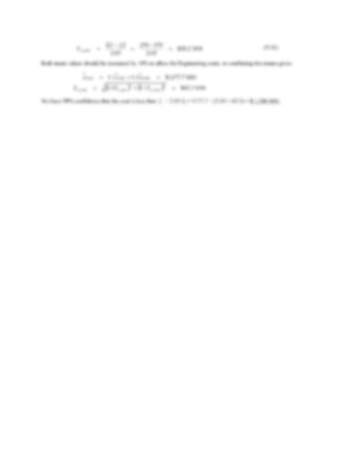
Solution 7.9
The ISBL cost on a Jan 2006 USGC basis was found to be $206.5 million in Example 7.8.
44
We can then develop the following table:
Country Location factor ISBL cost ($MM)
Solution 7.10
The equipment was entered into Aspen Process Economic Analyzer and costed on a Jan 2010 basis with the
following results:
45
Chapter 8
Solution 8.1
We can begin by putting all the costs onto the same basis. Although the answer is per scf of gas, it will be more
One gallon = 3.785 × 10⁻³ m3, so the pump work required per Mscf = 2.2 × 3.785 × 10-3 × 58.5 × 105 = 48.7 kJ/Mscf.
$4/MMBtu at time of writing. There are, of course, other costs in gas cleaning.
Solution 8.2
This problem is most easily solved using a spreadsheet to add up the fixed and variable production costs. The
template spreadsheet given in the online material at booksite.Elsevier.com/Towler was used (which is also given in
Example 8.2 – see Figure 8.13). Some additional calculations and assumptions were needed, as follows.
Electricity price – assumed to be $0.06/kWh.
Note that 1734/1988 = 87% of the cash cost of production is raw materials. Note also, that when an annual capital
charge is included (giving TCOP $2416/t), the breakdown of costs per metric ton product is:
Raw materials 1734 71.8%
46
Solution 8.3
As with problem 8.2 and Example 8.2, this is most easily solved by using a spreadsheet to track all the variable and
fixed costs of production. The plant fixed capital cost can be taken from the solution to problem 7.10. The following
additional calculations and assumptions were made.
48
Project Name
Project Number Sheet 1
2.90 289.91
22.87 2287.17
Gross Profit
Total Cost of Production
Company Name
Methyl Ethyl Ketone (Problem 8.3)
49
Solution 8.4
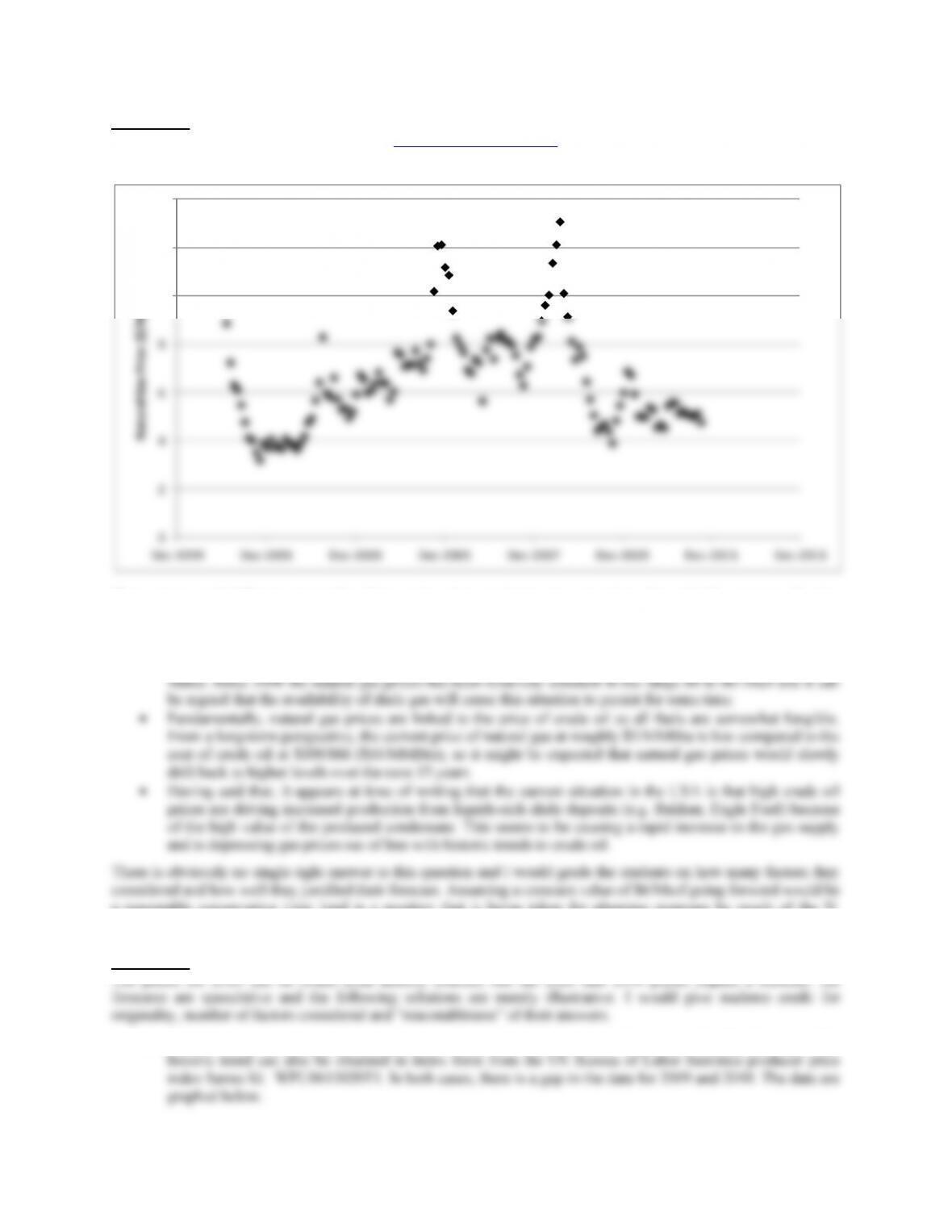
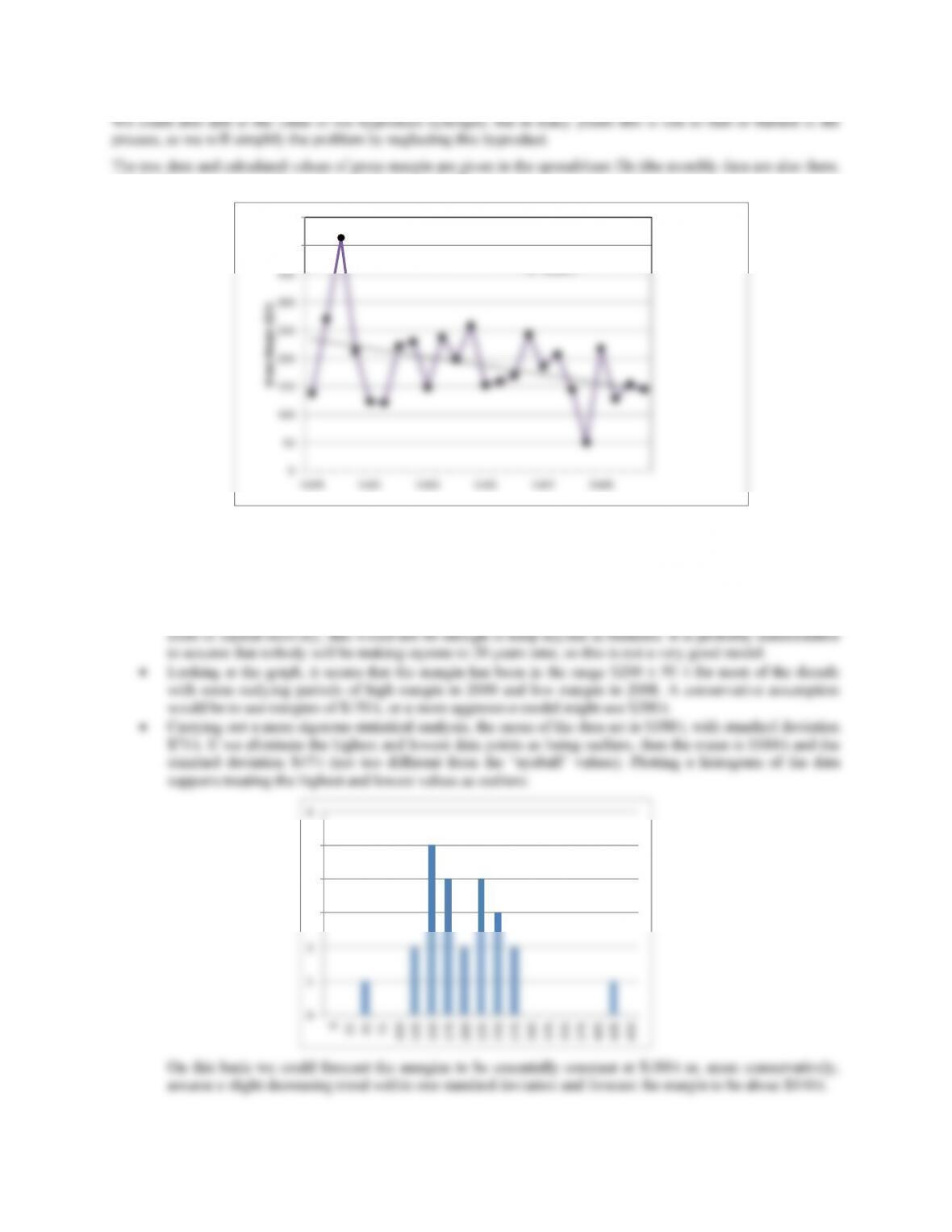
Natural gas prices can be downloaded from www.eia.gov/dnav/ng/hist. I used the “industrial” price set, which can
be obtained in spreadsheet format with data from 2001 to 2011. The raw data are shown below:
here are several different approaches that can be taken to forecasting gas prices forward 15 years (see Section
ave recently dropped as a result of the greater availability of shale gas in the United
0
2
4
6
8
10
12
14
Dec‐1999 Dec‐2001 Dec‐2003 Dec‐2005 Dec‐2007 Dec‐2009 Dec‐2011 Dec‐2013
NaturalGasPrice($/Mscf)
T
8.3.3), and the base data set will of course continue to evolve. At the time of writing (end of 2011), the following
factors should be considered:
• Industrial gas prices h
a reasonable conservative view (and is a position that is being taken for planning purposes by much of the N.
American chemical industry at the time of writing).
olution 8.5S
The prices for 2010 can be found from historic sources, but the 2020 and 2030 prices require a forecast. All
Economics Handbook series. The
graphed below.
forecasts are speculative and the following solutions are merely illustrative. I would give students credit for
originality, number of factors considered and “reasonableness” of their answers.
a) Sulfuric acid. I downloaded historic prices from the SRI Chemical
50
70
80
Sulfuricacid
downward trend in sulfuric acid prices over the next twenty years:
b) Sodium hydroxid . I took data from the SRI CEH report (converted to $/metric ton from
Once again, the price spike in 2008 was probably an aberration and was quickly corrected during the 2008-
2010 recession. Sodium hydroxide production costs are dominated by the cost of electricity, which has
historically been very flat (particularly in regions with low cost electricity, which is where chlor-alkali
plants tend to be located). The variation in sodium hydroxide prices is therefore tied to fluctuations in
during the 2008-2010 recession. Sulfuric acid is produced as a byproduct of fuel desulfurization and there
is a net global surplus of sulfur from which the acid is made. A reasonable assumption would be to see a
continuing slight
2010 $55/t
e (aka caustic soda)
$/short ton), but also available in Chemical Week and at the US BLS Series ID:
WPU06130302. The data are shown below.
the same data are
0
100
200
300
400
500
600
700
800
1998 2000 2002 2004 2006 2008 2010 2012
900
SodiumHydroxide
be argued that recent prices are a bubble caused by Asian demand that will soon be displaced by production
51
caustic prices as a cost, I would take a conservative position and use $400/t for 2020 and 2030.
Activated carbon. The SRI CEH report on activated carbon has 2009 prices ranging from $1.87 to $8.27
/kg, depending on the grade of carbon. The report lists both export and import prices. The import prices
c)
It can be seen that the prices seem to be drifting upwards, but I tried a linear regression and the regression
e prices would be $2.74/kg in 2020 and $3.19/kg in 2030.
d)
Solution
plotted the export prices to give the chart below.
using the linear correlation shown, th
Deionized water. The production of deionized water is discussed in Section 3.2.7, where it is stated that the
cost is roughly double the cost of raw water, i.e., typically about $1.0 per metric ton. Since the cost of
y=0.0452x‐ 88.566
R²=0.4338
0
0.5
1
1.5
2
2.5
3
1998 2000 2002 2004 2006 2008 2010 2012
$perkg
Activatedcarbon
8.6
T
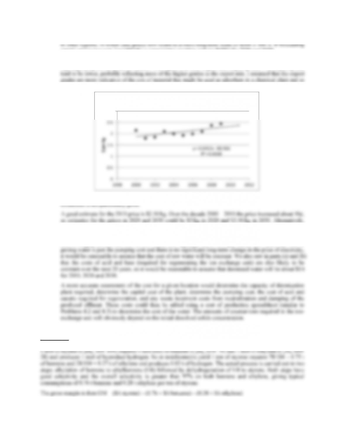
o determine the gross margin we need to know the yield of styrene from benzene and ethylene. From stoichiometry,
52
A linear trend line was added and it can be seen from the low regression coefficient that although margins appear to
be decreasing over time, there is not a strong correlation of the data.
To forecast the variation in styrene margin over the period 2010 to 2030 we could do any of the following:
y allowance for utilities, consumables, fixed
which allows you to run a larger data set if interested). The plot of gross margin against time is:
450
y=‐3.8683x+236.64
R²=0.1477
400
0
50
100
150
200
250
300
350
1H99 1H01 1H03 1H05 1H07 1H09
GrossMargin($/t)
• Use the linear regression through the data plotted above, in which case in 2030 (x = 52, two data points per
year) the margin will be $35/t. Since we have not made an
53
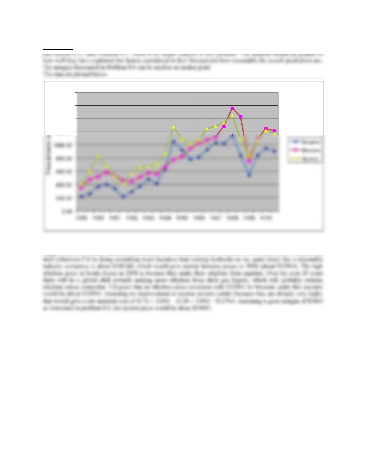
Solution 8.7
Overall, the benzene and ethylene prices move in line with crude oil (as might be expected), while the styrene
margin trend was already analyzed in problem 8.6. Guessing the value of crude oil in 20 years time is beyond my
skill (otherwise I’d be doing something more lucrative than writing textbooks in my spare time), but a reasonable
industry consensus is about $140/bbl, which would give similar benzene prices to 2008 (about $1200/t). The high
ethylene price in South Korea in 2008 is because they make their ethylene from naphtha. Over the next 20 years
there will be a global shift towards making more ethylene from shale gas liquids, which will probably restrain
ethylene prices somewhat. I’d guess that an ethylene price consistent with $1200/t for benzene under this scenario
would be about $1300/t. Assuming no improvement in styrene process yields (because they are already very high),
that would give a raw material cost of (0.76 × 1200) + (0.28 × 1300) = $1276/t. Assuming a gross margin of $184/t
as forecasted in problem 8.6, the styrene price would be about $1460/t.
0.00
800
1000.
1200.00
1400.00
1600.00
1800.00
1H99 1H00 1H01 1H02 1H03 1H04 1H05 1H06 1H07 1H08 1H09 1H10
e ($/metric ton)
Ben zene
.00
00
400.00
600.00
Pric
200.00
Eth ylene
Styren e
54
Chapter 9
Solution 9.1
See section 9.7.1. This is a straightforward application of equation 9.25:
(
)
[
]
1
+
n
ii
Solution 9.2
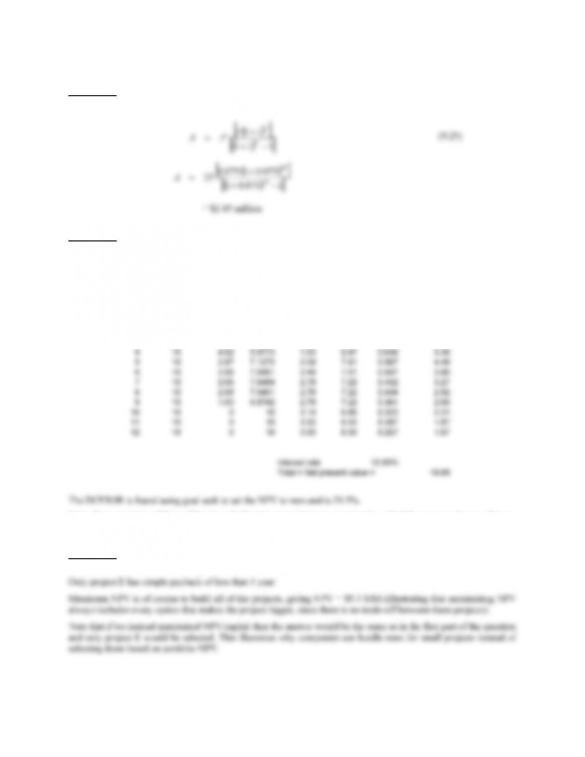
Refer to Example 9.4. This is easily solved using a spreadsheet (see below and spreadsheet file).
The NPV is $19.85 MM.
Note: the typesetting of this problem is such that the assumptions on construction schedule appear at the top of page
428. Some students might miss this and assume the plant is all built in year 0.
Solution 9.3
This problem is easily solved using a spreadsheet (see spreadsheet file and below).
Year Gross
profit
(MM$)
Depreciation
charge (MM$)
Taxable
income
(MM$)
Taxes
paid
(MM$)
Cash Flow
(MM$)
Discount
factor
Present
value of CF
(MM$)
0 0 0 0 0 -11.5 1 -11.5
1 0 0 0 0 -11.5 0.893 -10.27
2 10 3.29 6.7133 0 10.00 0.797 7.97
3 10 5.63 4.3673 2.35 7.65 0.712 5.45
55
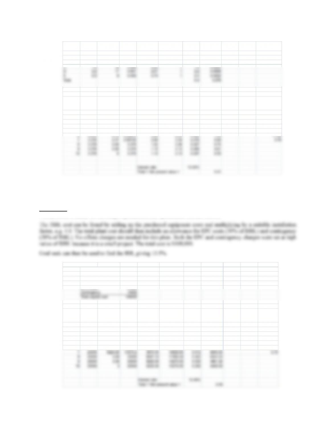
Note: anyone who gets the answer 5.2 instead of 5.3 used 7-yr MACRS instead of 5-yr (this is the way the problem
was posed in the 1st edition).
Solution 9.4
This problem is easily solved using a spreadsheet (see spreadsheet file and below).
Project Capex Fuel saved Savings Simple
Payback
Included? Capex Savings
(MM$) (MMBtu/h) (MM$/y) (y)
0.756
0.4536
Year Gross
profit
(MM$)
Depreciation
charge
(MM$)
Taxable
income
(MM$)
Taxes paid
(MM$)
Ca Flow
( $)
Discount
factor
Present
value of CF
(MM$)
1 0 0 0 0 -6.4 0.870 -5.57 5 yr MACRS
2 3.276 1. 0 3.28 0.756 2.48 20
3 3.276 2. 2.58 0.658 1.69 32
4 3.276 1.23 2.0472 0.43 2.85 0.572 1.63 19.2
5 3.276 0.74 2.53872 0.72 2.56 0.497 1.27 11.52
A 1.5 15 0.756 1.98 1 1.5
B 0.6 9 0.454 1.32 1 0.6
sh
MM
28 1.996
05 1.228 0.70
56
Solution 9.5
See Example 9.6.
The exchanger with carbon steel tubes should be selected as long as the plant turnaround schedule allows for
replacement of the tubes every two years without any loss in production (which would significantly increase the cost
of the first option).
Solution 9.6
The economic analysis spreadsheet from Example 9.5 can be modified with the new assumptions on investment cost
and capital recovery.
a) Cost of debt = 0.01, cost of equity = 0.40, so
b) With revised assumptions, NPV15 = $ - 154.3 MM (see sheet 9.6a)
57
Company Name
Project Name Adipic acid from phenol
Project Number Sheet 1
Address
Plant Location Units Metric
Case Description On Stream 8,000 hr/yr 333.33 day/yr
$MM/yr
Form XXXXX-Y Y-ZZ
Owner's Name
Solution 9.7
4
4
$MM Year % FC % WC % FCOP % VCOP
Main product revenue 560.0 ISBL Capital Cost 195.4 1 30% 0% 0% 0%
2 70% 0% 0% 0%
3 0% 100% 100% 50%
All figures in $MM unless indicated
Equity Cap Ex Revenue CCOP Gr. Profit Deprcn Taxbl Inc Tax Paid Cash Flow PV of CF NPV
511.7 48.3 0.0 48.3 16.9 31.4 0.1 -88.4
511.7 48.3 0.0 48.3 16.9 31.4 0.1 -88.3
0.0 48.3 16.9 31.4 0.1 -88.3
0.0 48.3 16.9 90.9 0.1 -88.1
pital Cost Basis Year 2010
China
REVENUES AND PRODUCTION COSTS CAPITAL COSTS
Ca
Byproduct revenue 4.4 OSBL Capital Cost 78.2
Raw materials cost 410.8 Engineering Costs 27.4
CASH FLOW ANALYSIS
Project year
1 56.4 0.0 0.0 0.0 0.0 0.0 0.0 -56.4 -40.3 -40.3
2 131.7 0.0 0.0 0.0 0.0 0.0 0.0 -131.7 -67.2 -107.5
17 0.0 560.0
18 0.0 560.0
19 0.0 560.0 511.7 48.3
20 -59.5 560.0 511.7 48.3
ECONOMIC ANALYSIS
Average cash flow 36.7 $MM/yr NPV 10 years -91.5 $MM IRR 10 years 4.8%
CONSTRUCTION SCHEDULE
58
Note that the contingency is 12.0% of the ISBL + OSBL fixed capital, which is about right for a class 2 estimate on
an established technology.
59


