
8-1
Chapter 8
Accounting for Long-Term Operational Assets
General Comments for Chapter 8
This chapter introduces the concepts of current, long-term, tangible, and intangible assets and
also explains how acquiring, using, and disposing of long-term operational assets affects fi-
nancial statements. Students are also introduced to the concepts of depreciation, depletion,
and amortization. Since these activities span several accounting periods, we recommend us-
ing a multicycle teaching model to illustrate accounting for them. Use a model that presents
financial statements vertically and accounting cycles horizontally. Students will see how de-
preciation accumulates on the balance sheet and how cash flows occur in different periods
from expense recognition. You can visually portray the connections between asset usage and
revenue generation. The multicycle model is a powerful classroom learning tool. Begin the
discussion by using a very simple example that students can understand. Most students un-
derstand that cars or trucks last for more than a year and that as the car or truck is driven, it
loses value becomes some portion of its life is ‘used up’. This helps them better understand
the concepts of depreciation, depletion, and amortization.
The chapter covers basket purchases, alternative depreciation computations, revising esti-
mates, relevant income tax considerations, and capital versus maintenance expenditures, as
well as depreciation, depletion, and amortization. Considerable effort has been devoted to
thinning the material into a manageable set of concepts that both accounting and general
business majors will find useful. For example, the text omits the sum-of-the-years’ digits
method and partial period depreciation.
Detailed Outline of a Lesson Plan for Chapter 8
I. Begin Chapter 8 by discussing the difference between current, long-term, tangi-
ble, and intangible assets. Explain that current assets are ones that will typically be
used within the coming 12 months or so and that long-term assets are ones that will
be used over several years. Tangible assets are ones that you can ‘touch and feel’ and
intangible assets are ones that you cannot see. Have students identify things that
would fall in to each asset category. Then ask students why the financial statements
would separate these assets into different categories. Leading such a discussion will
help students better relate to and identify those kinds of assets that would fall into
each category. Now would be a great time to discuss the fact that assets are generally
based on historical cost. Ask students why this would be the case. You can also
point out some of the debates around fair value accounting and ask students to com-
ment on the ease or difficulty around determining fair value for an asset that has been
in place for a few years or for an asset that might be unique to a company. Discus-
sions such as these bring ‘real world’ situations into the classroom and help even the

8-2
non-accounting majors understand how accounting information can be relevant to
their chosen major or to their life in general.
II. Work Demonstration Problem 8-1. This problem is based on a business that pur-
chases an automobile and then leases it to customers and illustrates three different de-
preciation methods across four years.
A. Begin the problem by briefly discussing how to determine asset cost. The
general rule is that the cost of an asset includes any expenditure reasonably neces-
sary to obtain the asset and get it ready to use. With respect to Demonstration
Problem 8-1 the automobile cost is $20,000 ($19,000 list – $1,000 cash discount +
$2,000 interior upgrade). The asset has a four-year useful life and a $4,000 sal-
vage value.
B. Scenario 1. Explain what is meant by depreciation and how this shows the ex-
pense associated with the use of a long–term asset. Explain what is meant by ‘sal-
vage value’ and that this represents the portion of the asset that will not be ‘used
up’. Next, have students calculate depreciation expense for each of the four years
using the straight-line method. Unless students have read the text, they will be
guessing at the answer (and assume that most of them have not read the text yet!).
Once students have had the chance to come up with their ideas of how straight–
line depreciation would be computed, ask them to share their ideas and then work
out the annual depreciation expense on the board so they can check their work.
The annual straight-line depreciation expense is $4,000 per year [($20,000 –
$4,000) ÷ 4].
After they have determined the straight-line depreciation expense, have stu-
dents prepare financial statements for the first accounting cycle. You can save
time by using the workpapers that accompany the demonstration problem. You
may also want to consider recording the events using the horizontal financial
statements model even though the problem does not require that they do so. Re-
cording the transactions in the horizontal financial statements model allows stu-
dents to see how these events aggregate into the financial statements. Computa-
tions for Scenario 1 (straight-line depreciation) are shown below:
Year 2015
1. Revenue. The problem specifies the 2015 revenue ($7,200).
2. Expense. The depreciation expense for 2015 is $4,000 (see computations
above). Have students fill in the amount of net income.
3. Cash. Determine the December 31, 2015 cash balance: cash increased by
$21,000 as a result of the stock issue. It decreased $20,000 with the automo-
bile purchase. Cash increased $7,200 with receiving rent revenue. Therefore,
the ending cash balance was $8,200 ($21,000 – $20,000 + $7,200).
4. Automobile. The cost of the car purchased was $20,000.

8-3
5. Accumulated Depreciation. At the end of the first year of operation, only
one year’s depreciation ($4,000) has been accumulated in this account. Have
students fill in the amount of total assets.
6. Common Stock. The business issued common stock for $21,000.
7. Retained Earnings. Since the business did not pay any dividends, the total
amount of net income was retained in the business. Retained earnings would
be $3,200. Have students verify total stockholders’ equity.
8. Cash Flows. Since revenue was collected in cash, the cash received from
customers was $7,200. Under investing activities there was a $20,000 outflow
to purchase the car, and there was a $21,000 financing inflow from issuing
stock. The net result was an $8,200 cash inflow. Since beginning cash was
zero, the ending cash balance is $8,200 ($8,200 + 0 = $8,200).
9. If students have trouble following the logic outlined above or if you want to
reinforce the logic, you can have students record the events for the first couple
of years in T-accounts.
Years 2016 − 2018
Income statements for these years are identical to the 2015 income statement.
Cash inflow from revenue is $7,200 each year. Since there are no cash expenses
(the only expense is depreciation), cash inflow from operating activities is $7,200
per year. The cash balance increases by $7,200 each year. For example, the cash
balance on the 2016 balance sheet is $15,400 ($8,200 beginning balance plus
$7,200 cash inflow from operating activities). The automobile is reported at cost
($20,000) for all years through 2018. Each year, accumulated depreciation in-
creases by the amount of depreciation expense ($4,000). Common Stock remains
unchanged at $21,000 on all balance sheets. Since there are no dividends, the
amount of retained earnings increases by the amount of net income reported each
year ($3,200).
Year 2019
The only event in 2019 is the sale of the auto for $4,300 cash. Since the book
value at the time of the sale is $4,000 ($20,000 cost – $16,000 accumulated depre-
ciation), the transaction results in a $300 gain. This is the only item reported on
the 2019 income statement. The ending cash balance is $34,100 ($29,800 begin-
ning balance plus $4,300 cash inflow from sale). Since the car was sold, the bal-
ance in the automobile and accumulated depreciation accounts is zero. Retained
earnings is $13,100 ($12,800 beginning balance plus $300 gain). The only item
on the statement of cash flows is the $4,300 inflow from investing activities re-
sulting from the sale of the auto.
C. Scenario 2. Before proceeding to Scenario 2 you will need to show your students
how to compute double-declining-balance depreciation. The computations are
shown below for your convenience:
Year
(Cost
─
Accumulated
x
(2 x Straight-
=
Depreciation

8-4
Depreciation)
Line Rate)
Expense
2015
($20,000
─
$ 0)
x
.5
=
$10,000
2016
(20,000
─
10,000)
x
.5
=
5,000
2017
(20,000
─
15,000)
x
.5
=
1,000*
2018
(20,000
─
16,000)
x
.5
=
0*
*The 2017 formula yields $2,500. However, only $1,000 can be charged
because the asset cannot be depreciated below its salvage value. Similar-
ly, the amount of depreciation recognized in 2018 is zero because the as-
set has been fully depreciated.
After you have shown students how to compute depreciation expense, have them
complete the financial statements. Again, using the workpapers will save class
time. Also, you may also want to consider recording the events in this scenario
using the horizontal financial statements model even though the problem does not
require that they do so. Recording the transactions in the horizontal financial
statements model allows students to see how these events aggregate into the fi-
nancial statements. We suggest you help the students get started by working
through the 2015 statements step by step. The logic for determining the amounts
on the statements is described above in the explanation for Scenario 1. Although
amounts for some items differ, the logic is the same.
Once the students have completed the financial statements, it is a good idea to
have them compare Scenario 2 statements with Scenario 1 statements. Point out
that the end result is the same under either method. The difference lies in the tim-
ing rather than the total amount of expense recognized. Also point out that the
double-declining balance depreciation scenario 2 required a larger amount of rev-
enue in the earlier years in order for the net income to be the same as was the case
for straight line depreciation scenario 1.
D. Scenario 3. Before proceeding to Scenario 3 you will need to show your students
how to compute units-of-production depreciation. The computations are shown
below for your convenience:
Begin by determining the depreciation cost per mile:
(Cost – Salvage Value) ÷ Number of Miles = Depreciation Cost Per Mile
($20,000 – $4,000) ÷ 100,000 = $0.16 per mile
Determine the annual depreciation expense by multiplying the number of miles
driven during the year by the depreciation cost per mile.
Year
Miles Driven
x
Cost Per Mile
=
Depreciation Expense
2015
30,000
x
0.16
=
$4,800
2016
10,000
x
0.16
=
1,600

8-5
2017
40,000
x
0.16
=
6,400
2018
25,000
x
0.16
=
3,200*
*The 2018 formula yields $4,000. However, only $3,200 can
be charged because the asset cannot be depreciated below its
salvage value.
After you have shown students how to compute depreciation expense, have them
complete the financial statements. Again, help them get started by working
through the 2015 statements step by step. At this point, students may be able to
just substitute the depreciation expense and accumulated depreciation amounts in
the prior financial statements without needing to record all events using the hori-
zontal financial statements model. The logic for determining the amounts on the
statements is described above in the explanation for Scenario 1. Although
amounts for some items differ, the logic is the same. Students are likely to need
less help for this scenario than they needed before.
Once the students have completed the financial statements, it is a good idea to
have them compare the financial statements generated under all three scenarios.
Emphasize that the end result is the same regardless of depreciation method. The
difference lies in the timing rather than the total amount of expense recognized.
This is also a good time to discuss why depreciation expense in some scenarios
was $0, even though the asset was still in use. It’s a good time to discuss how an
asset’s useful life is estimated by using historical information, industry averages,
or manufacturer’s estimates and that, as an estimate, it’s not always exactly cor-
rect. Explain that accumulated depreciation is a contra account associated with
long-term assets. If you have already covered Chapter 7, you may want to remind
students that they first encountered contra accounts when discussing allowance
for doubtful accounts. Since accumulated depreciation is a contra account associ-
ated with long-term assets, an asset’s book value would be the sum of the balance
in the asset account less the balance in the accumulated depreciation account.
Point out that an asset’s book value should never be lower than the estimated sal-
vage value.
III. Demonstration Problem 8-2 introduces accounting for capital expenditures and
maintenance costs incurred after the acquisition date. The objectives are twofold:
to illustrate how maintenance costs affect the financial statements differently than
capital expenditures and to show how capital expenditures made to improve the quali-
ty of an asset differ from those made to extend the useful life of the asset. The hori-
zontal financial statements model is suited to these instructional objectives. Draw or
display the horizontal financial statements model. Then show students how mainte-
nance costs and capital expenditures affect financial statements differently.
IV. Introduce accounting for natural resources. Highlight the similarities between
units-of-production depreciation and depletion. Use Exercise 8-19 A or B as a
demonstration problem.

8-6
V. Introduce accounting for intangible assets. Highlight the similarities between
straight-line depreciation and amortization computations. Use Exercise 8-20 A or B
as a demonstration problem.
VI. Time considerations and homework assignments. Plan to spend approximately
two hours of class time discussing depreciation and covering the different deprecia-
tion methods. Allow an additional hour to cover related subjects such as basket pur-
chases and accounting for capital expenditures, depletion, and amortization of intan-
gibles. Exercise 8-2 A or B requires students to distinguish between current and
long-term assets while Exercise 8-3 A or B requires students to identify tangible ver-
sus intangible assets. Problem 8-26 A or B requires students to compute and record
depreciation over multiple accounting cycles and can be used if you want your stu-
dents to see how depreciation affects financial statements over an asset’s life cycle.
Problem 8-27 A or B requires applying different depreciation methods to the same as-
set. Students will see that the amount of depreciation expense recognized in any sin-
gle accounting period is affected by the type of depreciation method chosen. Problem
8-32 A or B involves capital expenditures. Problem 8-34 A or B addresses amortiza-
tion of intangible assets.
8-7
Demonstration Problem 8-1 –Alternative Depreciation Methods
The following events pertain to Sanders Rental Company (SRC).
1. SRC was started when it issued common stock for $21,000 cash.
2. On January 1, 2015, SRC paid cash to purchase an automobile. The car dealer gave
Sanders a $1,000 cash discount off the $19,000 list price. However, Sanders paid an ad-
ditional $2,000 to equip the car with a more luxurious interior so it would have greater
appeal to his clientele. Sanders expected the car to have a four-year useful life and a
$4,000 salvage value. SRC expected to lease the car for 100,000 miles before disposing
of it.
3. SRC leased the car to a customer who drove it 30,000 / 10,000 / 40,000 / 25,000 miles
during 2015, 2016, 2017, and 2018, respectively. SRC sold the car on January 1, 2019,
for $4,300 cash.
4. Assume SRC recognized depreciation expense using one of three separate scenarios.
The revenue stream assumed for each scenario is shown below:
Revenue Stream
Scenario
2015
2016
2017
2018
1
$ 7,200
$7,200
$7,200
$7,200
2
$13,200
$8,200
$4,200
$3,200
3
$ 8,000
$4,800
$9,600
$6,400
Use the following depreciation method for each of the scenarios.
Scenario
Depreciation Method
1
Straight-line
2
Double-declining-balance
3
Units-of-production
Required
Prepare income statements, balance sheets, and statements of cash flows for 2015 through
2018 for each of the three scenarios.
8-8
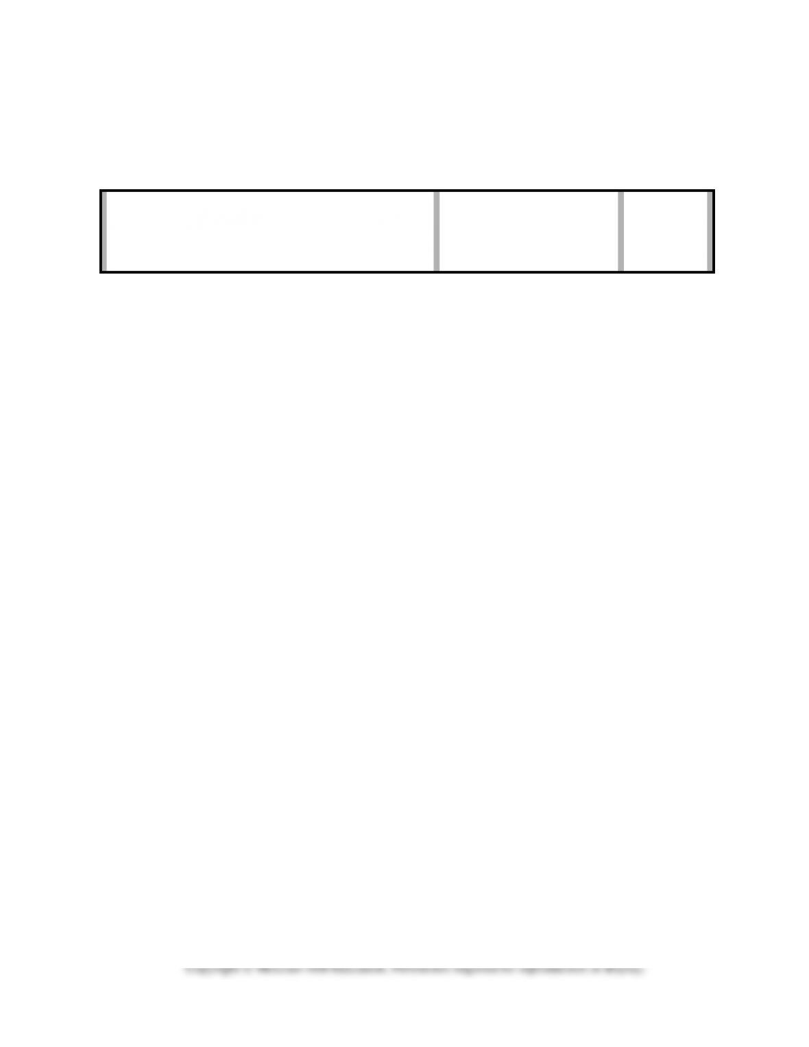
Demonstration Problem 8-2 – Capital vs. Revenue Expenditures
The following statements model depicts the financial condition of Boston Mechanical Com-
pany just prior to a $1,000 cash expenditure.
Assets
=
Liab.
+
Equity
Rev.
–
Exp.
=
Net Inc.
Cash Flow
Cash
+
Equip.
–
Accum.
Depr.
=
Ret. Earn.
1,000
+
5,000
–
2,000
=
0
+
4,000
0
–
0
=
0
0
Required
Show the effects of the expenditure on the statements model under the following three sepa-
rate scenarios.
1. The $1,000 was paid for maintenance cost.
2. The $1,000 was paid to improve the quality of the equipment.
3. The $1,000 was paid to extend the useful life of the equipment.
8-9
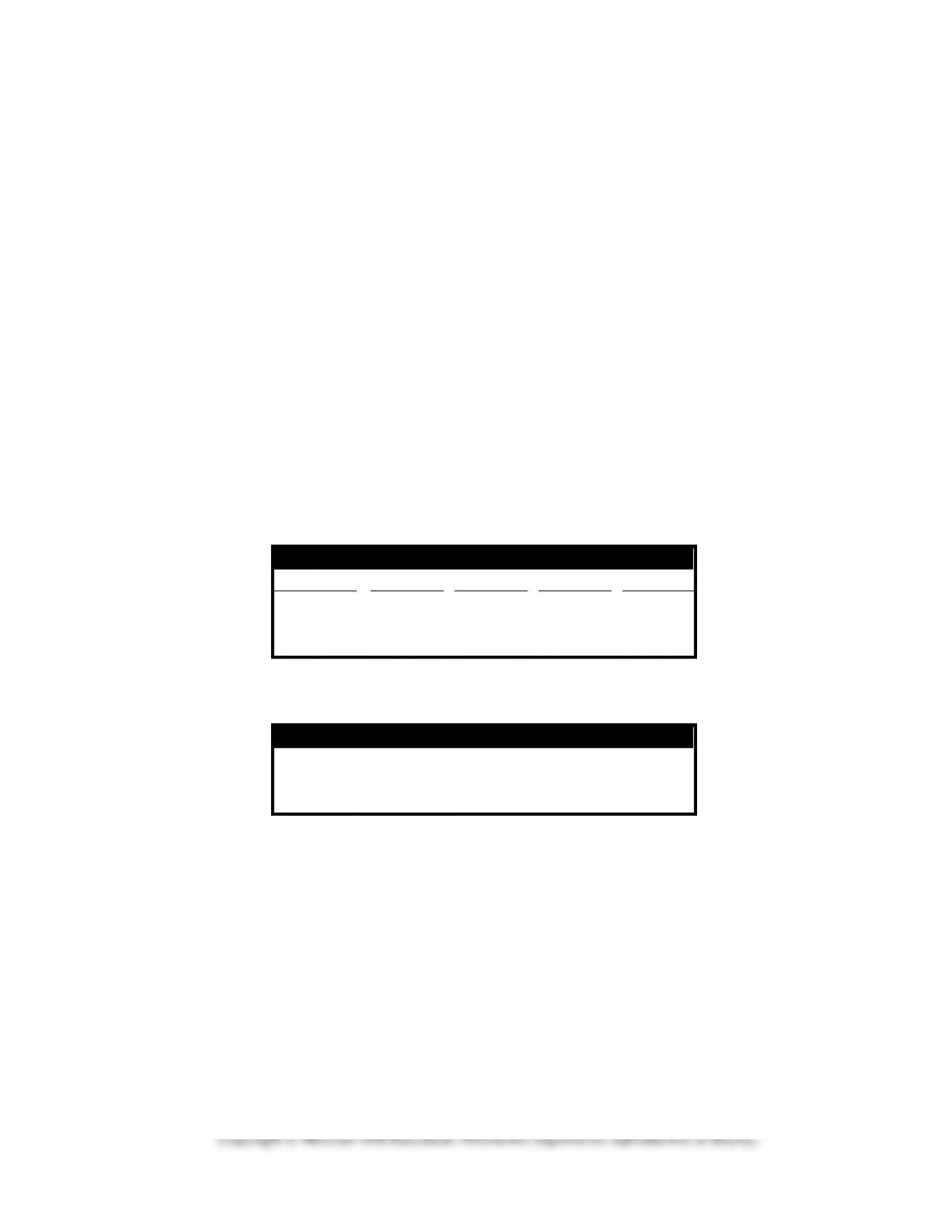
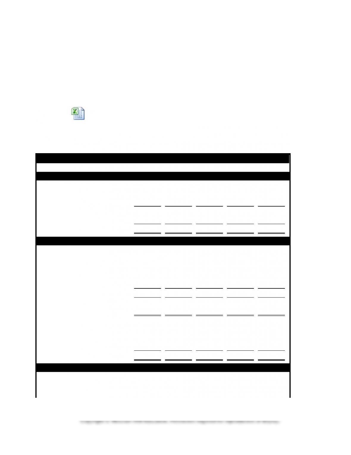
Demonstration Problem 8-1 Scenario 1 Solution
The embedded spreadsheet shows the transactions recorded using the horizontal
financial statements model. Even though the problem does not require students to
record transactions using the horizontal financial statements model, doing so helps
students link the transactions in the problem with the financial statements they are
required to prepare. You are welcome to skip this step if you think your students are
now able to link the described transactions to the required financial statements.
Worksheet Edmonds
FFAC9e Ch 8 IM DP8-
Straight-Line Depreciation
Income Statements
2015
2016
2017
2018
2019
Rent revenue
$7,200
$7,200
$7,200
$7,200
$ 0
Depreciation expense
4,000
4,000
4,000
4,000
0
Operating income
3,200
3,200
3,200
3,200
0
Gain on sale of automobile
0
0
0
0
300
Net income
$3,200
$3,200
$3,200
$3,200
$ 300
Balance Sheets
Assets
Cash
$ 8,200
$15,400
$22,600
$29,800
$34,100
Automobile
20,000
20,000
20,000
20,000
0
Accumulated depreciation
(4,000)
(8,000)
(12,000)
(16,000)
0
Book value, auto
16,000
12,000
8,000
4,000
0
Total assets
$24,200
$27,400
$30,600
$33,800
$34,100
Stockholders’ equity
Common stock
$21,000
$21,000
$21,000
$21,000
$21,000
Retained earnings
3,200
6,400
9,600
12,800
13,100
Total stockholders’ equity
$24,200
$27,400
$30,600
$33,800
$34,100
Statements of Cash Flows
Operating activities
Inflow from customer
$ 7,200
$ 7,200
$ 7,200
$ 7,200
$ 0
Investing activities
Outflow for automobile
(20,000)
8-10
Inflow from sale of auto
4,300
Financing activities
Inflow from stock issue
21,000
Net change in cash
8,200
7,200
7,200
7,200
4,300
Beginning cash balance
0
8,200
15,400
22,600
29,800
Ending cash balance
$ 8,200
$15,400
$22,600
$29,800
$ 34,100
8-11
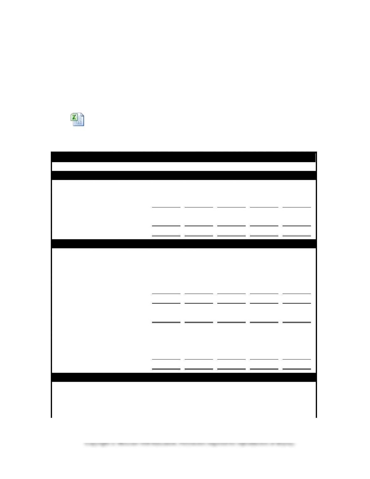
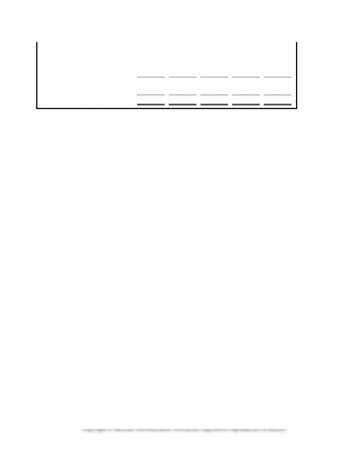
Demonstration Problem 8-1 Scenario 2 Solution
The embedded spreadsheet shows the transactions recorded using the horizontal
financial statements model. Even though the problem does not require students to
record transactions using the horizontal financial statements model, doing so helps
students link the transactions in the problem with the financial statements they are
required to prepare. You are welcome to skip this step if you think your students are
now able to link the described transactions to the required financial statements.
Worksheet Edmonds
FFAC9e Ch 8 IM DP8-
Double-Declining-Balance Depreciation
Income Statements
2015
2016
2017
2018
2019
Rent revenue
$13,200
$8,200
$4,200
$3,200
$ 0
Depreciation expense
10,000
5,000
1,000
0
0
Operating income
3,200
3,200
3,200
3,200
0
Gain on sale of automobile
0
0
0
0
300
Net income
$ 3,200
$3,200
$3,200
$3,200
$ 300
Balance Sheets
Assets
Cash
$14,200
$22,400
$26,600
$29,800
$34,100
Automobile
20,000
20,000
20,000
20,000
0
Accumulated depreciation
(10,000)
(15,000)
(16,000)
(16,000)
0
Book value, auto
10,000
5,000
4,000
4,000
0
Total assets
$24,200
$27,400
$30,600
$33,800
$34,100
Stockholders’ equity
Common stock
$21,000
$21,000
$21,000
$21,000
$21,000
Retained earnings
3,200
6,400
9,600
12,800
13,100
Total stockholders’ equity
$24,200
$27,400
$30,600
$33,800
$34,100
Statements of Cash Flows
Operating activities
Inflow from customer
$13,200
$8,200
$4,200
$3,200
$ 0
Investing activities
8-12
Outflow for automobile
(20,000)
Inflow from sale of auto
4,300
Financing activities
Inflow from stock issue
21,000
Net change in cash
14,200
8,200
4,200
3,200
4,300
Beginning cash balance
0
14,200
22,400
26,600
29,800
Ending cash balance
$14,200
$22,400
$26,600
$29,800
$34,100
Copyright © McGraw-Hill Education. Permission required for reproduction or display.
8-13
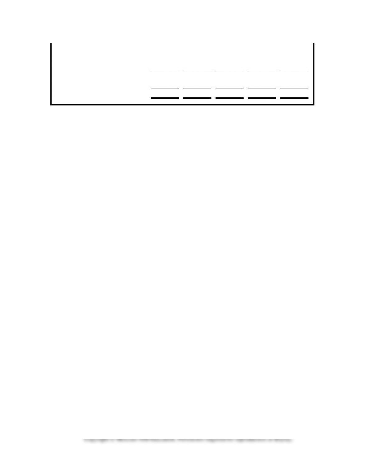
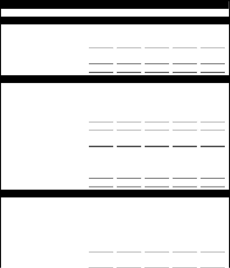
Demonstration Problem 8-1 Scenario 3 Solution
Note: While a horizontal financial statements model was presented to support the
solutions for scenarios 1 and 2, at this point the students should be able to discern
which fields on the financial statements below would change as a result of a change
in depreciation method. Therefore, there is not a horizontal financial statements
model presented for this scenario 3. Of course, you can create such a model if you
prefer to do so.
Units-of-Production Depreciation
Income Statements
2015
2016
2017
2018
2019
Rent revenue
$8,000
$4,800
$9,600
$6,400
$ 0
Depreciation expense
4,800
1,600
6,400
3,200
0
Operating income
3,200
3,200
3,200
3,200
0
Gain on sale of automobile
0
0
0
0
300
Net income
$3,200
$3,200
$3,200
$3,200
$ 300
Balance Sheets
Assets
Cash
$ 9,000
$13,800
$23,400
$29,800
$34,100
Automobile
20,000
20,000
20,000
20,000
0
Accumulated depreciation
(4,800)
(6,400)
(12,800)
(16,000)
0
Book value, auto
15,200
13,600
7,200
4,000
0
Total assets
$24,200
$27,400
$30,600
$33,800
$34,100
Stockholders’ equity
Common stock
$21,000
$21,000
$21,000
$21,000
$21,000
Retained earnings
3,200
6,400
9,600
12,800
13,100
Total stockholders’ equity
$24,200
$27,400
$30,600
$33,800
$34,100
Statements of Cash Flows
Operating activities
Inflow from customer
$ 8,000
$ 4,800
$ 9,600
$ 6,400
$ 0
Investing activities
Outflow for automobile
(20,000)
Inflow from sale of auto
4,300
Financing activities
Inflow from stock issue
21,000
Net change in cash
9,000
4,800
9,600
6,400
4,300
Beginning cash balance
0
9,000
13,800
23,400
29,800