
5-1
Chapter 5
Accounting for Inventories
General Comments for Chapter 5
This chapter explains inventory valuation methods, how to determine cost of goods sold, and
other accounting issues related to inventory. It shows students that a company may report
certain assets in financial statements at different amounts depending on the accounting meth-
ods chosen. For example, a company using the FIFO method will report inventory at a dif-
ferent value than it would if it used LIFO. Students learn that companies experiencing com-
parable economic events can report balance sheet and income statement data that differ sig-
nificantly. It may be the accounting principles chosen rather than economic conditions that
affect the amounts reported in the financial statements. Since asset valuation affects expense
recognition, this chapter offers opportunities to emphasize the relationship between the bal-
ance sheet and the income statement.
Be alert to the inconsistency between the acronyms FIFO and LIFO and computing the end-
ing inventory balance. The acronyms refer to the amount of product cost expensed as cost of
goods sold on the income statement. FIFO means the costs of the first items purchased are
the first costs to be charged to cost of goods sold. Since the number of units sold is usually
much larger than the number of units in ending inventory, it is quicker to indirectly calculate
cost of goods sold by computing the amount of ending inventory and then subtracting that
amount from cost of goods available for sale. So we often teach students to calculate the
ending inventory amount. This approach creates an inconsistency between the cost flow ac-
ronyms and the computations; the acronyms refer to cost of goods sold and the computations
focus on ending inventory.
If you value comprehension over faster computations, compute cost of goods sold in a man-
ner consistent with the acronyms, namely by multiplying the number of units sold by the cost
per unit. Although this approach requires more arithmetic, the benefits derived from logical
consistency are worth the effort. This method is also consistent with the way companies
keeping perpetual inventory records practice. Cost of goods sold is computed as sales occur.
If you would like to begin the chapter with a problem-based learning exercise, see the notes
below.
Problem-Based Learning Case: Inventory Cost
Instructions: The case appears on the following page in a format you can copy or display.
Distribute copies of the case to the class before providing any explanation of alternate inven-
tory costing methods. Ask students to read the case and individually develop answers. After
allowing students time to develop their individual answers, put them into groups to reach
5-2
consensus on an answer. Also, ask each group to select a spokesperson. Allow groups time
to develop answers, then call on some of the spokespersons to share their solutions. As you
respond to the student solutions, explain the basic concepts of inventory cost flow assump-
tions. Emphasize the concept of gross margin.
The possible answers are:
FIFO
LIFO
WAVG
Sales revenue
$40
$40
$40
Cost of goods sold
(25)
(31)
(28)
Gross margin
15
$9
$12
Other operating expenses
(5)
(5)
(5)
Net income
$10
$4
$7
Chapter 5 Problem-Based Learning Case: Inventory Cost
John Smith purchased two toy cars to resell. The cars were identi-
cal in every respect except that John purchased them at different
times for different costs. The first car purchased cost $25. The
second one purchased cost $31. John sold one of the cars for $40.
John’s other operating expenses were $5. Based on this infor-
mation alone, what was John’s net income?
Detailed Outline of a Lesson Plan for Chapter 5
5-3
I. Two factors affect the complexity of product cost allocations: (1) the number of
layers of inventory and (2) the number of units in each layer. The simplest model has
two layers with only one product in each layer. Start your explanation at this level.
Introduce Demonstration Problem 5-1 by telling your students that a furniture store
owns two beds which are identical with respect to appearance, quality, and brand
name. However, the store purchased the beds at different times for different prices.
The first bed cost the store $400; the second bed cost $450. The store sold one of the
beds for $600, and the store manager cannot identify which of the beds it was. First,
review how gross margin is computed. Then, instruct your students to compute the
gross margin on the sale. Be patient while they struggle for a while. Your objective
is for them to discover the problem before you provide a solution. Given a reasonable
length of time, someone is likely to subtract the average cost [($400 + $450) ÷ 2 =
$425] from the sales price ($600) to get a gross margin of $175. When this happens,
identify this method as weighted average and broaden the subject to include FIFO and
LIFO. Write the solution on the board as follows:
FIFO
LIFO
Weighted
Average
Sales
600
600
600
Cost of goods sold
(400)
(450)
(425)
Gross margin
200
150
175
In this simplified context you can make the critical points that distinguish each meth-
od from the others. For example, tell your students to assume that three different
companies use the different cost flow methods. Company A uses FIFO, Company B
LIFO, and Company C weighted average. Then ask which company is the best per-
former. Most students will choose FIFO because of the higher reported gross margin.
Of course, all three are the same. Each company experienced exactly the same eco-
nomic events. The only difference is in how they reported the events. You may also
want to point out that, in an inflationary economy, LIFO produced the lowest gross
margin. This is a good time to discuss the tax implications of FIFO versus LIFO.
We suggest you provide a follow-up exercise by creating an alternative two-layer sin-
gle-product problem. Have the students work this problem in class to make sure they
know how to apply the different approaches before you move on to more complex
problems that include multiple layers with differing prices.
II. Demonstration Problem 5-2 introduces accounting for inventories with multiple
layers and prices. The objective here is to show students how cost flow methods dif-
fer from each other. For example, does FIFO or LIFO produce a higher gross mar-
gin? The horizontal financial statements model is not suited to this type of analysis
because we are not interested in comparing statements (e.g., does an event affect the
income statement differently than the statement of cash flows?). Instead, we want to
5-4
see how different cost flow methods affect a particular statement (e.g., what does the
income statement look like under FIFO, LIFO, and weighted average?).
You can easily illustrate the distinction between cost of goods sold under FIFO versus
LIFO in a multilayer example. Draw a picture of a barrel on the board. Show differ-
ent layers of inventory piling up in the barrel. For FIFO, draw a hole in the bottom of
the barrel. Explain that the first items in inventory are the first ones out (sold). Then
erase the hole in the bottom of the barrel and replace it with a hole in the top of the
barrel. Removing inventory items from the top illustrates LIFO. The illustration be-
low is labeled to match the inventory available in Demonstration Problem 6-2.
Have your students complete Demonstration Problem 5-2 using a vertical format to
prepare income statements, balance sheets, and statements of cash flows. If your stu-
dents have trouble going directly to preparing statements, you may have them first
record the events in T-accounts or using the horizontal financial statements model.
Once they have prepared the statements, have them make the following observations.
A. Notice that the cost flow method does not affect revenue.
B. Have the students verify that the amount of cost of goods sold plus ending inven-
tory is equal to the amount of cost of goods available for sale. In other words, the
total product cost is the same for all cost flow methods. The difference lies in
how the cost is allocated between cost of goods sold and ending inventory.
C. With the exception of tax consequences, cash flow is not affected by the cost flow
method.

5-5
III. The text covers accounting for inventories when purchases and sales occur in–
termittently. If you include this subject, you may use Exercise 5-8A or B as a
demonstration problem and Exercise 5-9A or B as a follow-up problem.
IV. Use Demonstration Problem 5-3 to show students how to write down inventory
to lower of cost or market. Use the horizontal financial statements model to illus-
trate the effect of the write-down on the financial statements.
V. The text covers the gross margin method of estimating the ending inventory bal-
ance. Use Exercise 5-12 A or B to illustrate this approach to inventory estimation.
VI. Use Exercise 5-14 A or B to illustrate the effects of inventory misstatements on
the elements of financial statements.
VII. Time considerations and homework assignments. Allot approximately one class
hour to inventory topics. Students seem to grasp the inventory cost flow concepts
relatively easily when the method of calculating cost of goods sold is presented in a
manner consistent with the cost flow acronyms. Problem 5-19 A or B provides good
follow-up to Demonstration Problem 5-2. Problem 5-20 A or B can be used as
homework to reinforce the lower of cost or market concepts illustrated in Demonstra-
tion Problem 5-3. Problem 5-21 A or B provides practice estimating ending invento-
ry. As with other chapters, you will not have time to cover everything. Choose what
you deem appropriate. Avoid assigning too much. Unrealistically high expectations
demotivate students and discourage learning.

5-6
Demonstration Problem 5-1 – Inventory Cost Issue
A furniture store inventory includes two beds that are identical with respect to appearance,
quality, and brand name. However, the store purchased the beds at different times for differ-
ent prices. The first bed cost the store $400, and the second bed cost $450. Assume the store
sells one of the beds for $600. Also assume the store manager cannot identify which bed was
sold.
Required
Determine the gross margin on the sale of the bed.
Demonstration Problem 5-2 – Inventory Cost Flow Assumptions
Crystal Apple Sales Company began 2015 with cash of $2,000, inventory of $3,600 (200
crystal apples that cost $18 each), $2,500 of common stock, and $3,100 of retained earnings.
The following events occurred during 2015.
1. Crystal Apple purchased additional inventory twice during 2015. The first purchase
consisted of 800 apples that cost $20 each, and the second consisted of 1,200 apples that
cost $24 each. The purchases were on account.
2. The company sold 2,040 apples for cash at a selling price of $40 each.
3. The company paid $44,800 cash on accounts payable for inventory purchases.
4. Crystal Apple paid $26,000 cash for operating expenses.
Required
a. Record the events in ledger T-accounts or using the horizontal financial statements mod-
el using the three different cost flow assumptions: FIFO, LIFO, and weighted average.
b. Prepare an income statement, a balance sheet, and a statement of cash flows under each
of the three cost flow assumptions.
5-7
Demonstration Problem 5-3 – Lower of Cost or Market for Inventory
Pleasant Grove Electronics carries four different types of calculators. The quantities, costs,
and market values are shown below. Based on this information, determine the necessary
lower of cost or market (LCM) write-down assuming Pleasant Grove determines LCM on an
individual basis. Use a horizontal financial statements model to show how the write-down
would affect the balance sheet, income statement, and statement of cash flows.
Type
Quantity
Unit
Cost
Unit
Market
A
100
$12.00
$15.00
B
550
8.00
6.00
C
710
25.00
24.00
D
240
20.00
22.00
5-8
Demonstration Problem 5-1 Solution
FIFO
LIFO
Weighted
Average
Sales
600
600
600
Cost of goods sold
(400)
(450)
(425)
Gross margin
200
150
175
5-9
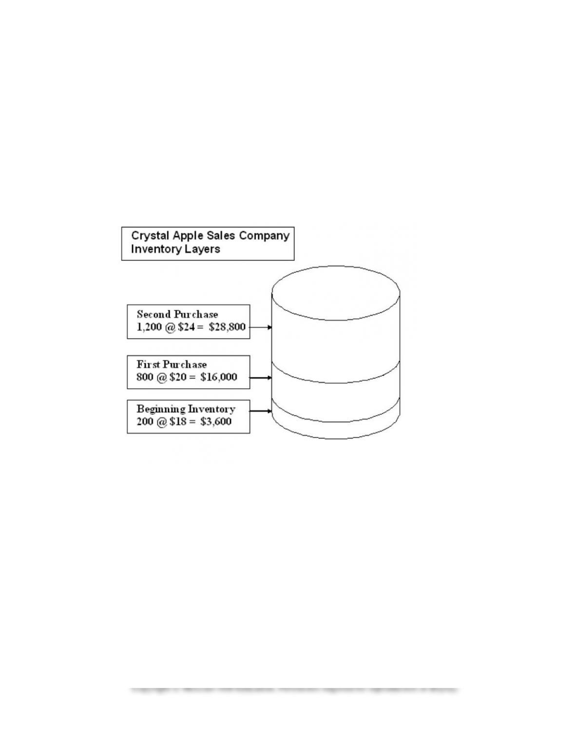
Demonstration Problem 5-2 Solution, Inventory Summary
Crystal Apple’s 2015 inventory contains the following layers.
Units
Cost per Unit
Total Cost
Beginning balance
200
x
$18
=
$ 3,600
First purchase
800
x
20
=
16,000
Second purchase
1,200
x
24
=
28,800
Total available
2,200
$48,400
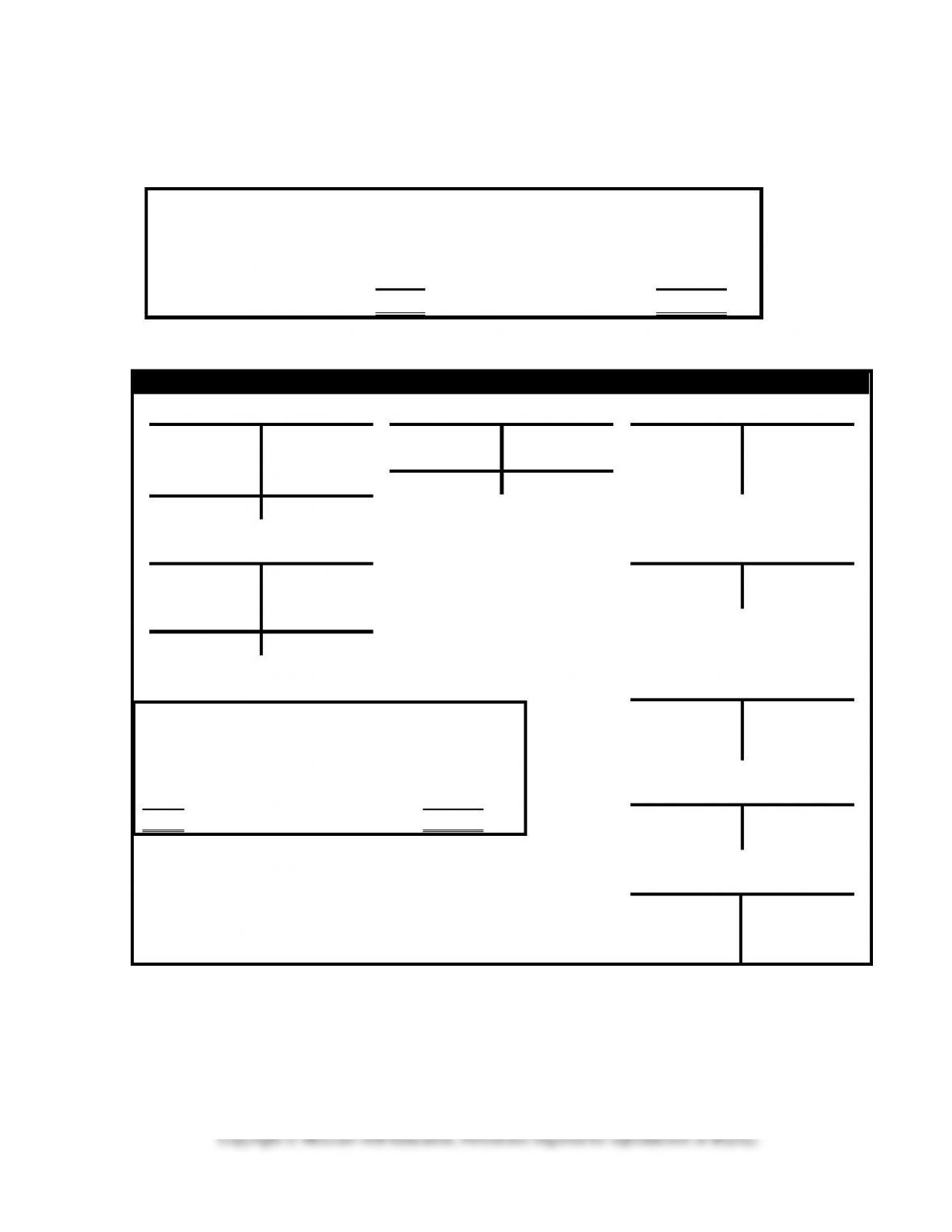
Demonstration Problem 5-2 Solution, part a. Ledger T-accounts
Ledger T-Accounts – FIFO Cost Flow
Cash
Accounts Payable
Common Stock
Bal. 2,000
44,800 (3)
(3) 44,800
16,000 (1a)
2,500 Bal.
(2a) 81,600
26,000 (4)
28,800 (1b)
0 Bal.
Bal. 12,800
Inventory
Retained Earnings
Bal. 3,600
44,560 (2b)
3,100 Bal.
(1a) 16,000
(1b) 28,800
Bal. 3,840
Sales Revenue
81,600 (2a)
Cost of Goods Sold
(2b) 44,560
Operating Expenses
(4) 26,000
Computation of Cost of Goods Sold using FIFO
Units
Cost per Unit
Total Cost
200
x
$18
=
$ 3,600
800
x
20
=
16,000
1,040
x
24
=
24,960
2,040
$44,560
5-10
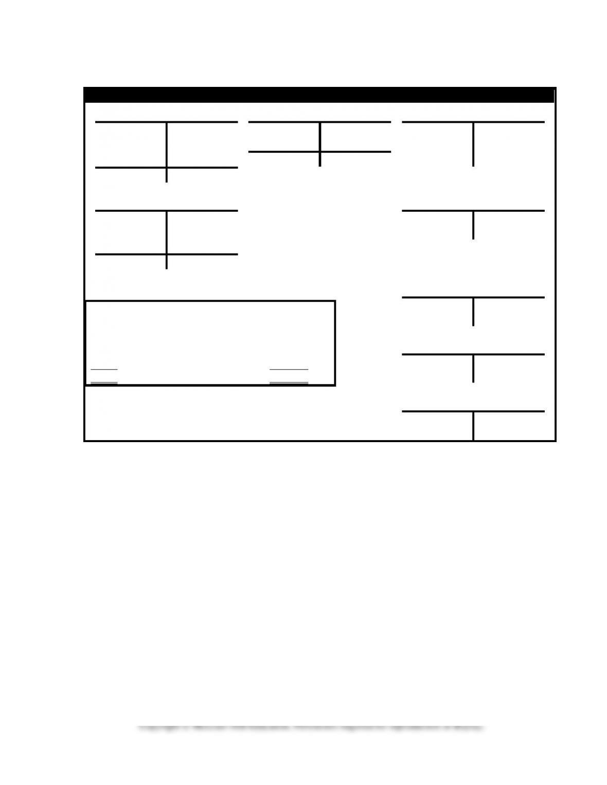
Demonstration Problem 5-2 Solution, part a. Ledger T-accounts
Ledger T-Accounts – LIFO Cost Flow
Cash
Accounts Payable
Common Stock
Bal. 2,000
44,800 (3)
(3) 44,800
16,000 (1a)
2,500 Bal.
(2a) 81,600
26,000 (4)
28,800 (1b)
0 Bal.
Bal. 12,800
Inventory
Retained Earnings
Bal. 3,600
45,520 (2b)
3,100 Bal.
(1a) 16,000
(1b) 28,800
Bal. 2,880
Sales Revenue
81,600 (2a)
Cost of Goods Sold
(2b) 45,520
Operating Expenses
(4) 26,000
Computation of Cost of Goods Sold using LIFO
Units
Cost per Unit
Total Cost
1,200
x
$24
=
$28,800
800
x
20
=
16,000
40
x
18
=
720
2,040
$45,520
5-11
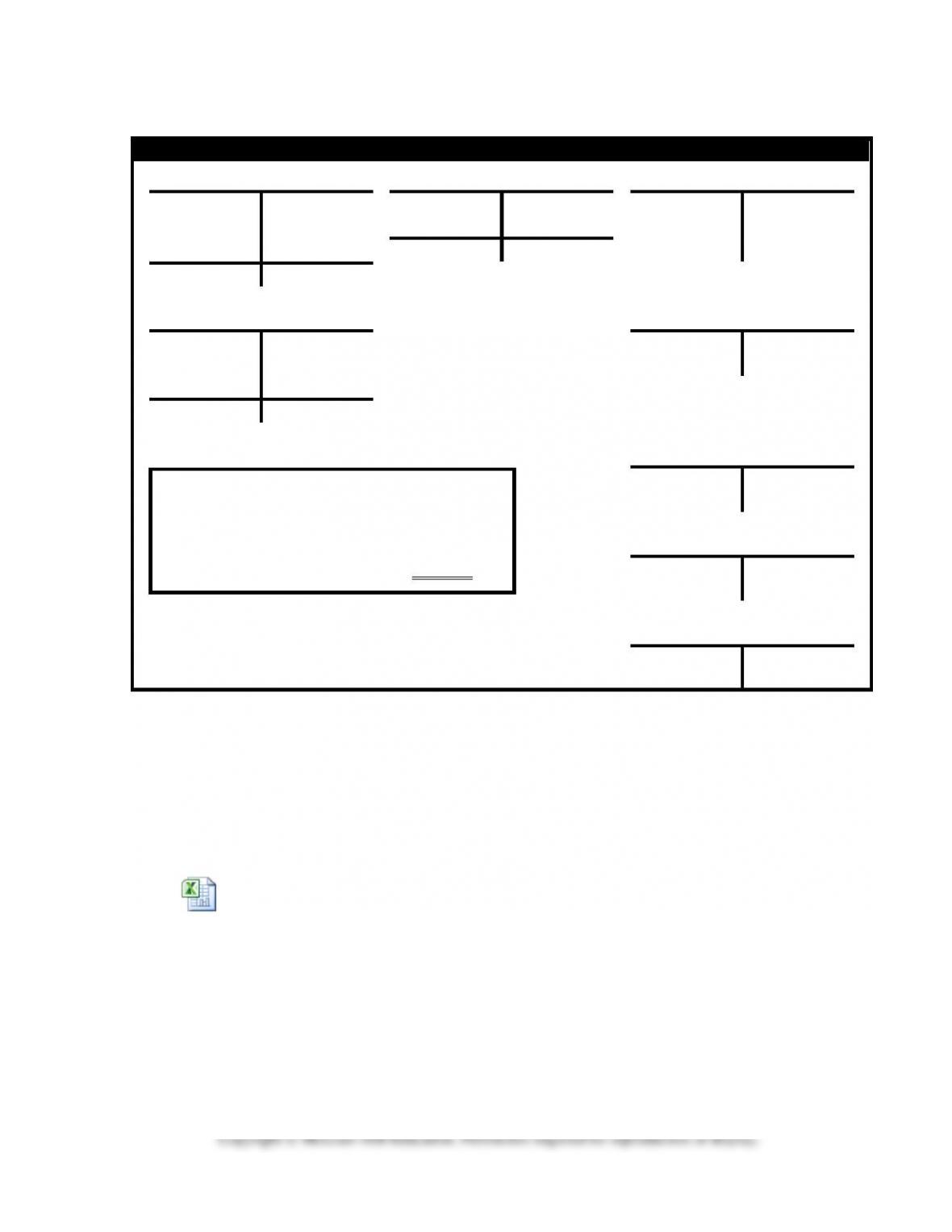
Demonstration Problem 5-2 Solution, part a. Ledger T-accounts
Ledger T-Accounts – Weighted Average Cost Flow
Cash
Accounts Payable
Common Stock
Bal. 2,000
44,800 (3)
(3) 44,800
16,000 (1a)
2,500 Bal.
(2a) 81,600
26,000 (4)
28,800 (1b)
0 Bal.
Bal. 12,800
Inventory
Retained Earnings
Bal. 3,600
44,880 (2b)
3,100 Bal.
(1a) 16,000
(1b) 28,800
Bal. 3,520
Sales Revenue
81,600 (2a)
Cost of Goods Sold
(2b) 44,880
Operating Expenses
(4) 26,000
Demonstration Problem 5-2 Solution, part a. Horizontal Financial
Statements Model
Worksheet Edmonds
FFAC9e Ch 5 IM.xls
Computation of Cost of Goods Sold using WA
Cost per Unit = $48,400 ÷ 2,200 units = $22
Units
Cost per Unit
Total Cost
2,040
x
$22
=
$44,880
Copyright © McGraw-Hill Education. Permission required for reproduction or display.
5-12
Demonstration Problem 5-2 Solution, part b. Financial Statements
Crystal Apple Sales Company
Comparative Financial Statements
Income Statements for the Year Ended December 31, 2015
FIFO
LIFO
Wt. Avg.
Sales
$81,600
$81,600
$81,600
Cost of goods sold
(44,560)
(45,520)
(44,880)
Gross margin
37,040
36,080
36,720
Operating expenses
(26,000)
(26,000)
(26,000)
Net Income
$11,040
$10,080
$10,720
Balance Sheets at December 31, 2015
Assets
FIFO
LIFO
Wt. Avg.
Cash
$12,800
$12,800
$ 12,800
Inventory
3,840
2,880
3,520
Total assets
$16,640
$15,680
$16,320
Stockholders’ equity
Common stock
$ 2,500
$ 2,500
$ 2,500
Retained earnings
14,140
13,180
13,820
Total stockholders’ equity
$16,640
$15,680
$16,320
Statements of Cash Flows for the Year Ended December 31, 2015
Cash flow from oper. activities
FIFO
LIFO
Wt. Avg.
Cash inflow from customers
$81,600
$81,600
$81,600
Cash outflow for inventory
(44,800)
(44,800)
(44,800)
Cash outflow for oper. exp.
(26,000)
(26,000)
(26,000)
Net cash inflow from oper. act.
10,800
10,800
10,800
Cash flow from investing act.
0
0
0
Cash flow from financing act.
0
0
0
Net increase in cash
10,800
10,800
10,800
Beginning cash balance
2,000
2,000
2,000
Ending cash balance
$12,800
$12,800
$12,800