Unlock document.
This document is partially blurred.
Unlock all pages and 1 million more documents.
Get Access
Serial Problem — SP 6, Success Systems (concluded)
2.
Per Unit
Total
Total
LCM Applied
Inventory Items
Units
Cost
Market
Cost
Market
To Items
Office productivity ........
3
$ 76
$ 74
$228
$222
$222
Desktop publishing ......
2
103
100
206
200
200
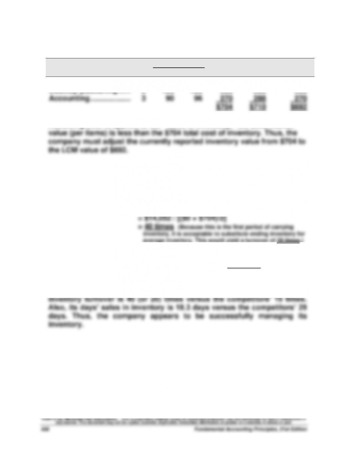
Accounting ....................
3
90
96
270
288
270
$704
$710
$692
Assuming LCM is applied to the “items of inventory,” the $692 market
Part B
1. Ratio computations for the three months ended March 31, 2014:
Inventory Turnover = Cost of Goods Sold / Average Inventory
Days’ Sales in Inventory = (Ending Inventory/Cost of Goods Sold) x 365
= ($704 / $14,052) x 365 = 18.3 days
2. Success Systems outperforms its competitors on both ratios. Its
Reporting in Action — BTN 6-1
($ thousands for all parts)
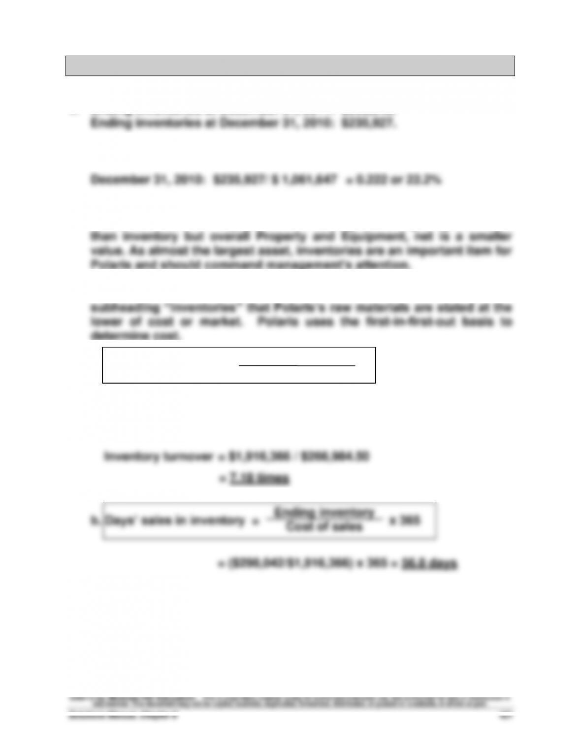
1. Ending inventories at December 31, 2011: $298,042.
2. December 31, 2011: $298,042/$1,228,024 = 0.243 or 24.3%
3. Polaris’s inventories are its second largest assets (behind cash) at
December 31, 2011. Equipment and tooling has a higher gross value
4. Reviewing notes to its financial statements, we see Note 1 under the
5. a. Inventory turnover =
Average inventory = ($298,042 + $235,927)/2
= $266,984.50
6. Solution depends on the financial statement information obtained.
Cost of sales
Average inventory
Comparative Analysis — BTN 6-2
($ thousands)
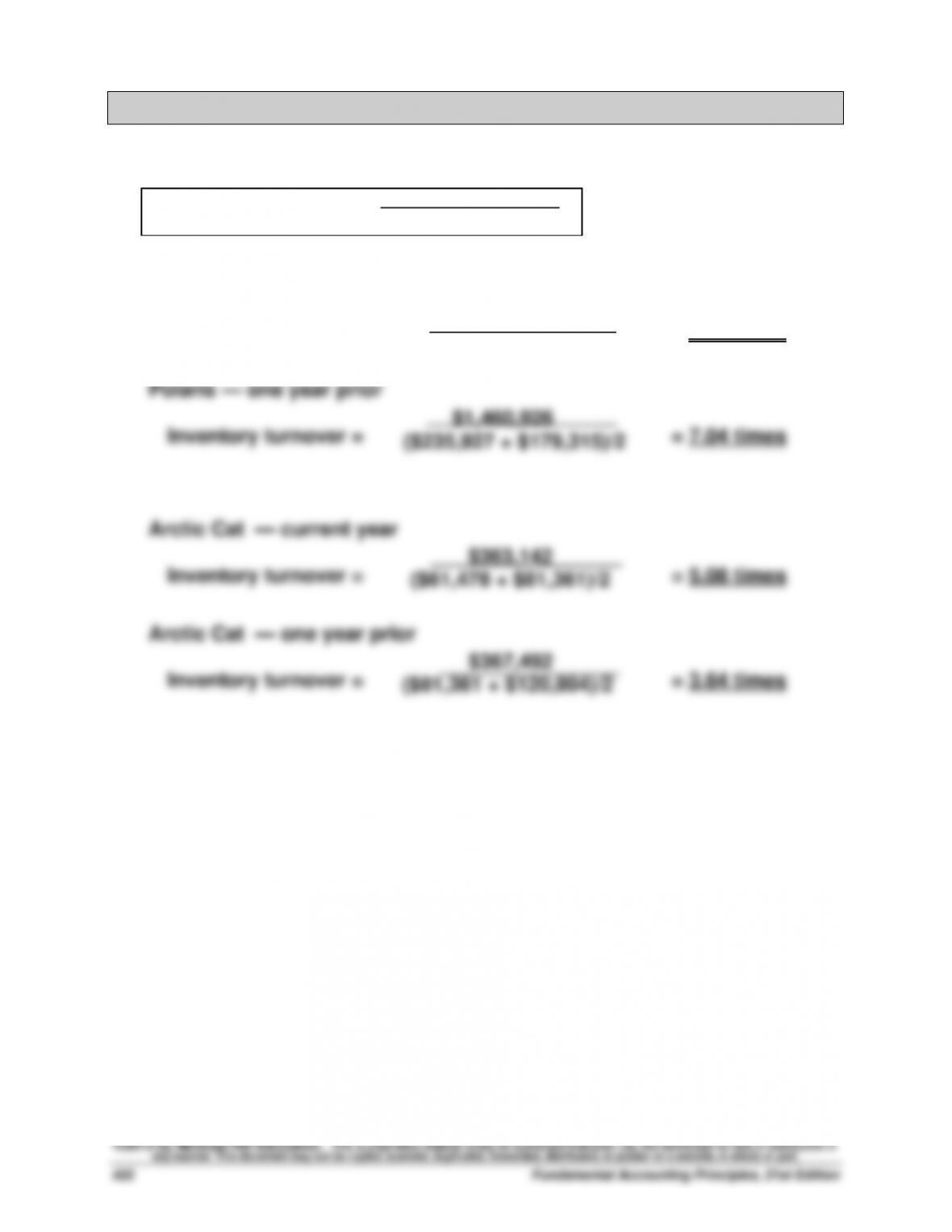
1. Inventory turnover =
Polaris — current year
Inventory turnover = = 7.18 times
Cost of sales
Average inventory
$1,916,366
($298,042 + $235,927)/2
Comparative Analysis (Concluded)
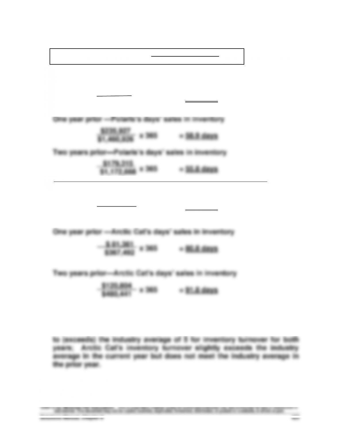
2. Days’ sales in inventory = x 365
Current year — Polaris’s days’ sales in inventory
x 365 = 56.8 days
Current year — Arctic Cat’s days’ sales in inventory
x 365 = 61.8 days
3. For all years examined here, Polaris manages its inventory more
efficiently than does Arctic Cat. Polaris’s inventory turnover is higher,
and its days’ sales in inventory is shorter. Polaris compares favorably
Ending Inventory
Costs of Goods Sold
$298,042
$1,916,366
$61,478
$363,142
$1,172,668
Ethics Challenge — BTN 6-3
1. Profit Margin: In an economic environment of rising costs, the use of
FIFO results in a lower cost of goods sold than LIFO. If cost of goods
sold is lower, then net income will be higher. A higher net income will
2. First, it is true that managers have discretion in choosing an inventory
costing method. It appears, however, that Golf Challenge’s owner does
not understand that changing methods can only be done very
Third, the full disclosure principle requires the owner to disclose to the
bank that the company has implemented a change in inventory costing
method from LIFO to FIFO.
Communicating in Practice — BTN 6-4
[Note: An acceptable memorandum format should be used.]
The body of the memo would likely recommend use of the LIFO method for
this start-up business. The memo should explain that this would allow for
the matching of the most recent (higher) costs against revenue through
Taking It to the Net — BTN 6-5
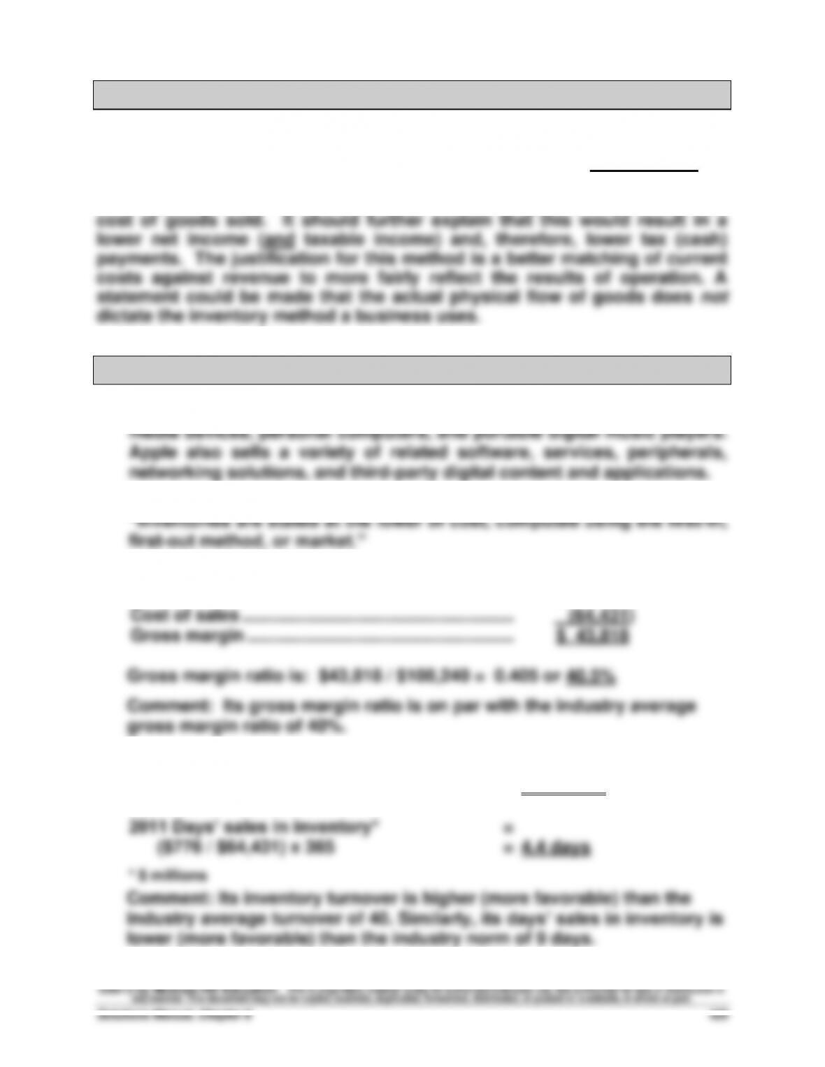
1. Apple designs, manufactures, and markets mobile communication and
2. Its summary of significant accounting policies (Note 1) reports:
3. Its gross margin for 2011 is ($ millions)
Sales .....................................................................
$108,249
Cost of sales ........................................................
(64,431)
Gross margin .......................................................
$ 43,818
Gross margin ratio is: $43,818 / $108,249 = 0.405 or 40.5%
Comment: Its gross margin ratio is on par with the industry average
gross margin ratio of 40%.
4. 2011 Inventory turnover* =
$64,431/ [($776 + $1,051)/2] = 70.5 times
Teamwork in Action — BTN 6-6
Concepts and procedures to illustrate in expert presentation:
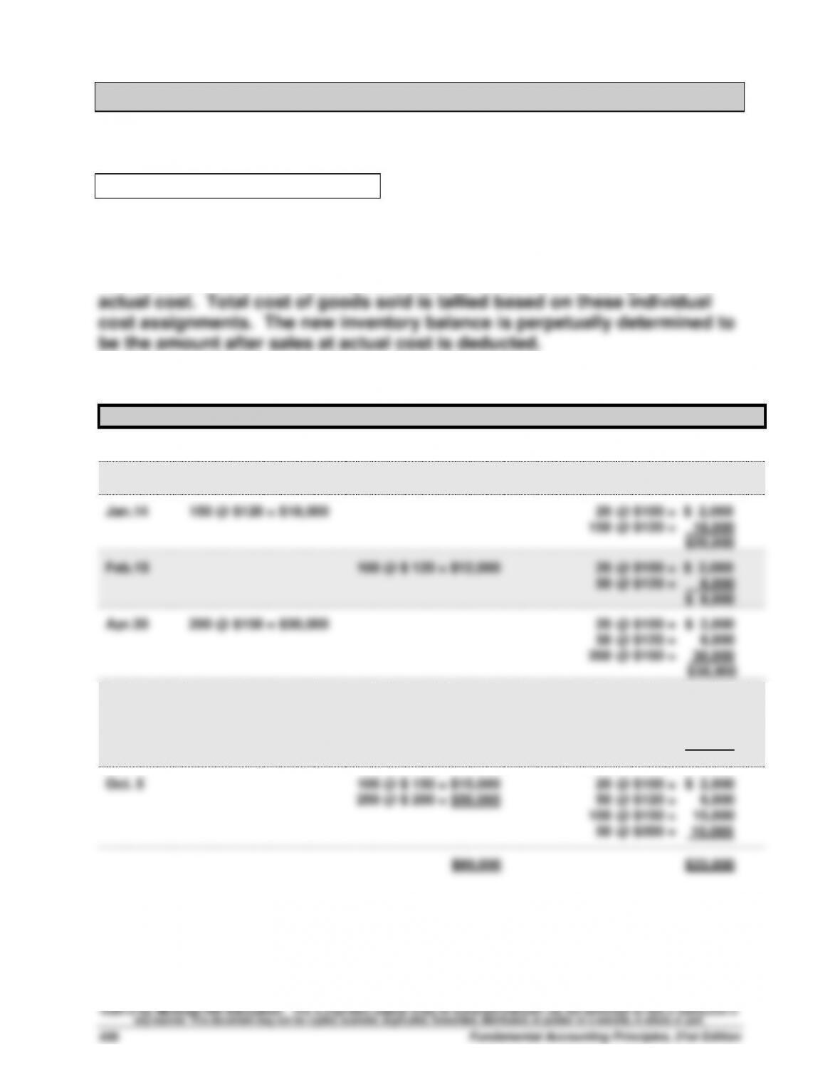
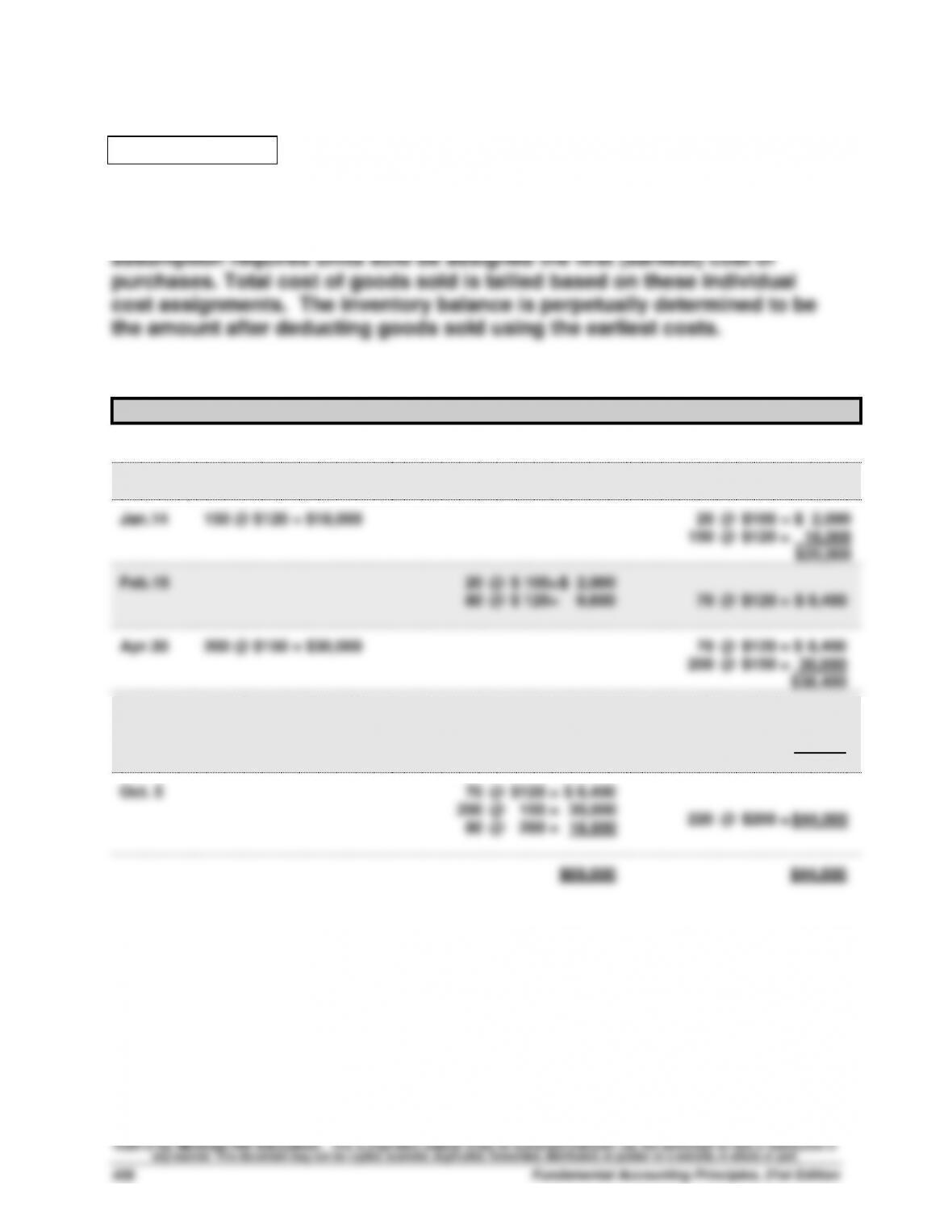
Specific Identification Expert:
(a) and (b) Concept:
Purchases are always recorded at the actual specific costs. The specific
identification cost flow assumption requires units sold be assigned their
(a) and (b) Procedures:
Date
Goods Purchased
Cost of Goods Sold
Inventory Balance
Jan. 1
50 @ $100 = $ 5,000
Jan.10
30 @ $ 100 = $ 3,000
20 @ $100 = $ 2,000
Jan.14
150 @ $120 = $18,000
20 @ $100 = $ 2,000
150 @ $120 = 18,000
$20,000
Feb.15
100 @ $ 120 = $12,000
20 @ $100 = $ 2,000
50 @ $120 = 6,000
$ 8,000
Apr.30
200 @ $150 = $30,000
20 @ $100 = $ 2,000
50 @ $120 = 6,000
200 @ $150 = 30,000
$38,000
Sept 26
300 @ $200 = $60,000
20 @ $100 = $ 2,000
50 @ $120 = 6,000
200 @ $150 = 30,000
300 @ $200 = 60,000
$98,000
Oct. 5
100 @ $ 150 = $15,000
250 @ $ 200 = $50,000
20 @ $100 = $ 2,000
50 @ $120 = 6,000
100 @ $150 = 15,000
50 @ $200 = 10,000
$80,000
$33,000
Teamwork in Action (Continued)
LIFO Expert:
(a) and (b) Concept:
Purchases are always recorded at actual costs. The LIFO cost flow
(a) and (b) Procedures:
Date
Goods Purchased
Cost of Goods Sold
Inventory Balance
Jan. 1
50 @ $100 = $ 5,000
Jan.10
30 @ $100 = $ 3,000
20 @ $100 = $ 2,000
Jan.14
150 @ $120 = $18,000
20 @ $100 = $ 2,000
150 @ $120 = 18,000
$20,000
Feb.15
100 @ $120 = $12,000
20 @ $100 = $ 2,000
50 @ $120 = 6,000
$ 8,000
Apr.30
200 @ $150 =$30,000
20 @ $100 = $ 2,000
50 @ $120 = 6,000
200 @ $150 = 30,000
$38,000
Sept 26
300 @ $200 = $60,000
20 @ $100 = $ 2,000
50 @ $120 = 6,000
200 @ $150 = 30,000
300 @ $200 = 60,000
$98,000
Oct. 5
300 @ $200 = $60,000
50 @ $150 = $ 7,500
______
20 @ $100 = $ 2,000
50 @ $120 = 6,000
150 @ $150 = 22,500
$82,500
$30,500
Teamwork in Action (Continued)
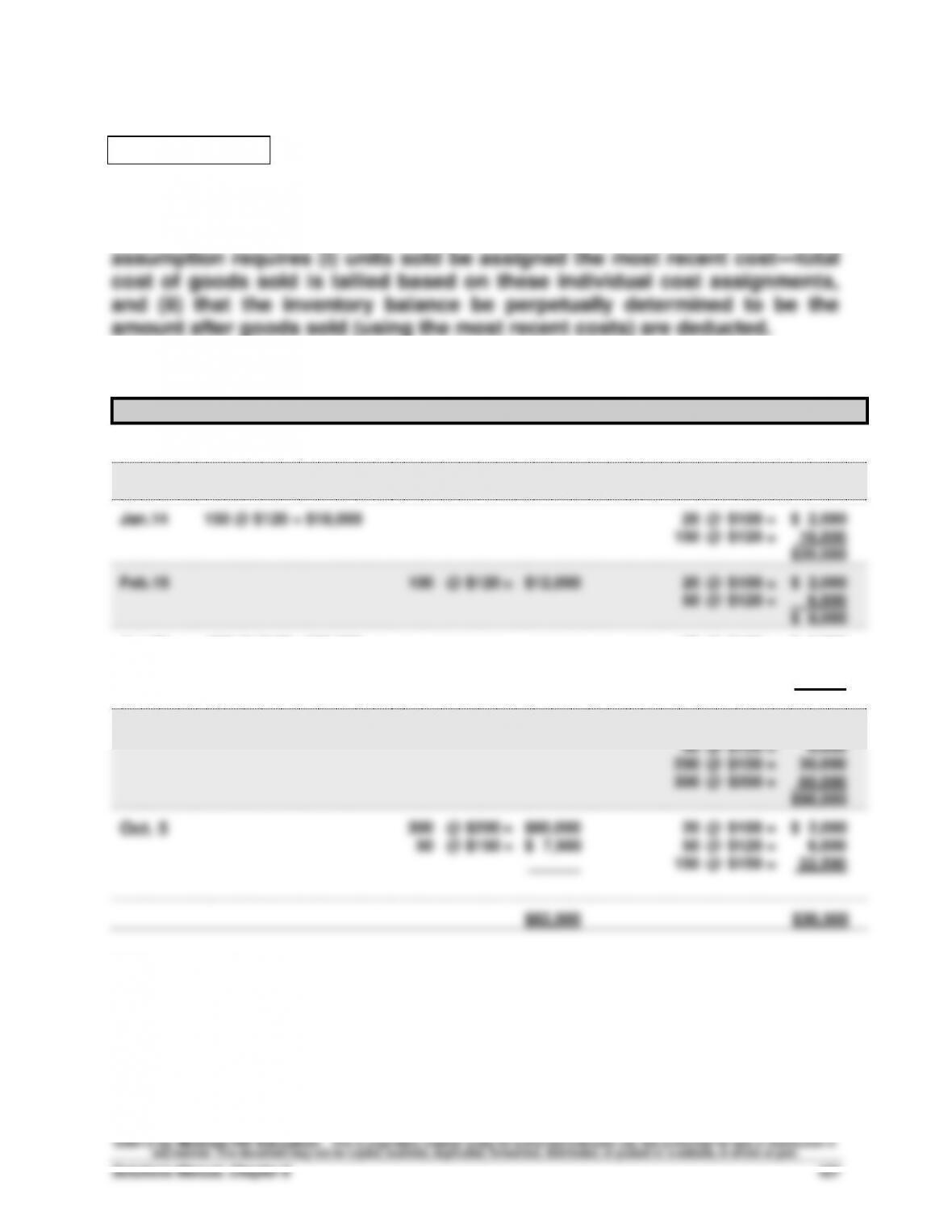
FIFO Expert:
(a) and (b) Concept:
Purchases are always recorded at actual costs. The FIFO cost flow
(a) and (b) Procedures:
Date
Goods Purchased
Cost of Goods Sold
Inventory Balance
Jan. 1
50 @ $100 = $ 5,000
Jan.10
30 @ $100 = $ 3,000
20 @ $100 = $ 2,000
Jan.14
150 @ $120 = $18,000
20 @ $100 = $ 2,000
150 @ $120 = 18,000
$20,000
Feb.15
20 @ $ 100= $ 2,000
80 @ $ 120= 9,600
70 @ $120 = $ 8,400
Apr.30
200 @ $150 = $30,000
70 @ $120 = $ 8,400
200 @ $150 = 30,000
$38,400
Sept 26
300 @ $200 = $60,000
70 @ $120 = $ 8,400
200 @ $150 = 30,000
300 @ $200 = 60,000
$98,400
Oct. 5
70 @ $120 = $ 8,400
200 @ 150 = 30,000
80 @ 200 = 16,000
220 @ $200 = $44,000.
$69,000
$44,000
Teamwork in Action (Continued)
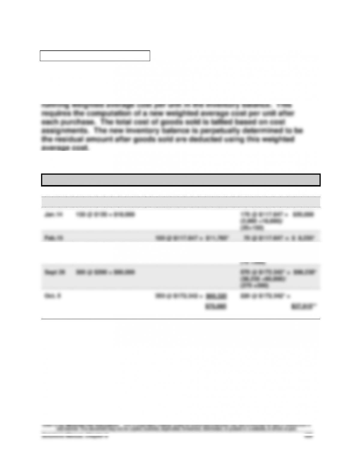
Weighted Average Expert:
(a) and (b) Concept:
Purchases are always recorded at actual costs. The Weighted Average
cost flow assumption requires units sold be assigned a cost based on
(a) and (b) Procedures:
Date
Goods Purchased
Cost of Goods Sold
Inventory Balance
Jan. 1
50 @ $100 = $ 5,000
Jan.10
30 @ $100 = $ 3,000
20 @ $100 = $ 2,000
Jan.14
150 @ $120 = $18,000
170 @ $117.647 = $20,000
(2,000 +18,000)/
(20+150)
Feb.15
100 @ $117.647 = $11,765*
70 @ $117.647 = $ 8,235*
Apr.30
200 @ $150 = $30,000
270 @ $141.611*= $38,235*
(8,235+30,000)/
(70 +200)
Sept 26
300 @ $200 = $60,000
570 @ $172.342* = $98,235*
(38,235 +60,000)/
(270 +300)
Oct. 5
350 @ $172.342 = $60,320
220 @ $172.342* =
$75,085
$37,915**
* rounded ** adjusted for rounding
Teamwork in Action (Concluded)
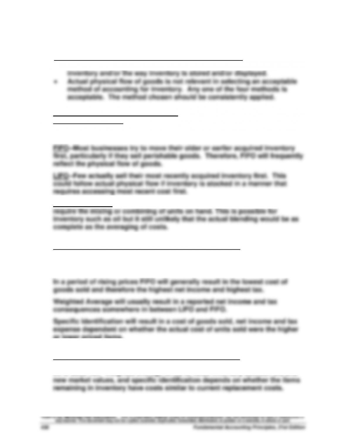
(c) Cost Flow versus Actual Physical Flow
Typical comments experts may express in response to (c):
• Physical flow of goods can be affected by the type of products in
More Specific Expert Comments to (c):
Specific Identification--Always reflects the actual cost flow. Electronic
scanning has increased the ability to use this method in businesses that sell
homogeneous goods.
Weighted Average--This cost is rarely the actual cost flow. This would
(d) Impact of Methods
Typical comments experts may express in response to (d):
In a period of rising prices LIFO will generally result in the highest cost of
goods sold and therefore the lowest net income and lowest tax. However,
LIFO must be used for financial reporting if it is used for tax purposes.
or lower priced items.
(e) Valuation
Typical comments experts may express in response to (e):
FIFO tends to value ending inventory closest to replacement cost whereas
LIFO does not. Weighted average tends to value inventory between old and
Entrepreneurial Decision — BTN 6-7
Part 1
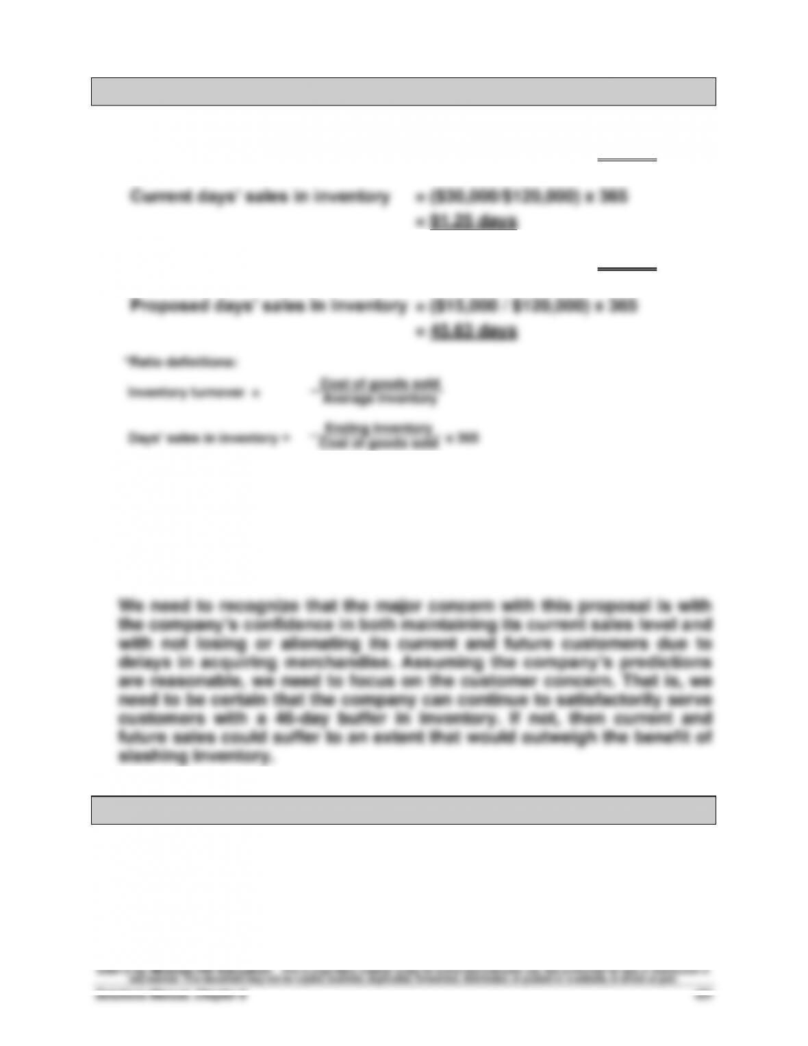
(a) Current inventory turnover = $120,000 / $30,000 = 4 times
(b) Proposed inventory turnover = $120,000 / $15,000 = 8 times
Part 2
The owners’ proposal for their company would yield a much improved
inventory turnover of 8 vis-à-vis the current turnover of 4. On the
downside, its days’ sales in inventory would dramatically decline from
91 days to 46 days. Assuming an inventory buffer of 46 days is
sufficient, then the proposal should be implemented.
Hitting the Road — BTN 6-8
There is no formal solution for this field activity. The required solution
does allow students to see the relevance of studying merchandise
activities and inventory accounting.
Cost of goods sold
Global Decision — BTN 6-9
1. Inventory turnover =
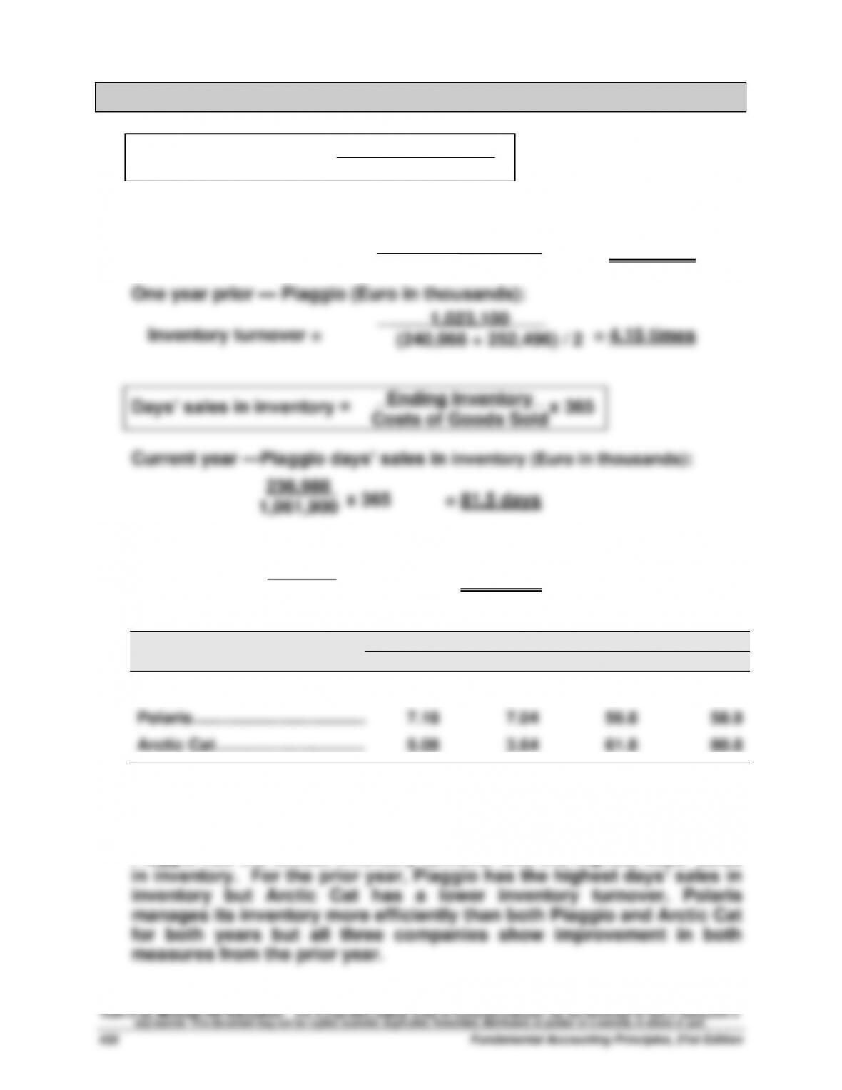
Current year — Piaggio (Euro in thousands):
Inventory turnover = = 4.45 times
One year prior—Piaggio days’ sales in inventory (Euro in thousands):
x 365 = 85.6 days
Inventory Turnover
Days’ Sales in Inventory
Company
Current
Prior Year
Current
Prior Year
Piaggio ...............................................
4.45
4.15
81.5
85.6
Polaris ................................................
7.18
7.04
56.8
58.9
Arctic Cat ................................
5.08
3.64
61.8
80.8
Note: Computations for Polaris and Arctic Cat are in BTN 6-2.
2. For the current year and prior years, Polaris has the highest inventory
turnover and the lowest days’ sales in inventory. For the current year,
Piaggio has the lowest inventory turnover and the highest days’ sales
Cost of sales
Average inventory
240,066
1,023,100
1,061,900
(236,988 + 240,066) / 2
1,061,900


