CHAPTER 25
25-2
Additional Information on Related Assignment Material
Connect (Available on the instructor’s course-specific website) repeats all numerical Quick Studies, all
Exercises and Problems Set A. Connect provides new numbers each time the Quick Study, Exercise or
Problem is worked. It allows instructors to monitor, promote, and assess student learning. It can be used
in practice, homework, or exam mode.
Corresponding problems in set B also relate to learning objectives identified in grid on previous page.
Problems 25-1A and 25-4A can be completed using EXCEL. The Serial Problem for Success Systems
starts in this chapter and continues throughout many chapters of the text. It is most readily solved
manually if you use the working papers that accompany text.
Synopsis of Chapter Revision
• Charlie’s Brownies: NEW opener with new entrepreneurial assignment
• Updated graphic on industry cost of capital estimates
• New discussion on outsourcing of information and technology services
• New presentation on payback periods for health care providers
• New discussion on link between CEO compensation and IRR
• Simplified computation of the accounting rate of return
• New example showing calculation of net present value with salvage value
• New exhibit showing formula for computing average investment
• Simplified discussions and exhibits for several examples of managerial decisions
• Enhanced graphics on NPV and IRR decision rules
Narrated PowerPoint Correlation Guide
Learning Objective
Slides
P1
3-7
P2
8-10
P3
11-14
P4
15-19
C1
20-22
A1
23-29
A2
40
Chapter Outline
Section 1⎯Capital Budgeting
Capital budgeting is the process of analyzing alternative long-term investments
and deciding which assets to acquired or sell. Fundamental goal of capital
budgeting decisions is to earn a satisfactory rate of return. Such decisions
require careful analysis, and are the most difficult and risky decisions made by
managers. Difficult because of need to make predictions of events that will
occur well into the future. Risky because outcome is uncertain, large amounts
of money are involved, long-term commitment is required, and decision may
be difficult or impossible to reverse. Several techniques are used to make
capital budgeting decisions.
3. To compute payback period, exclude all non-cash revenue and
expenses from computation.
a. When annual cash flows are even in amount,
Payback Period = Cost of Investment
(starting with the negative cash flow resulting from the
initial investment); when cumulative net cash flow
changes from positive to negative, the investment is fully
recovered. (see Exhibit 25.3)
4. Payback period should not be only consideration in evaluating
Notes
Chapter Outline
B. Accounting Rate of Return (or return on average investment)
1. Also called return on average investment; is computed by
dividing the projects after tax net income by the average
amount invested in it.
2. Accrual basis after-tax net income is used.
3. Compute the average investment:
a. If straight-line deprecation is used and there is zero
salvage value then:
Annual average = (Beg. Book Value + End. Book value)
Investment 2
b. If straight-line deprecation is used and there is a salvage
value then:
Annual average = (Beg. Book Value + Salvage Value)
similar lives and risk.
b. Capital investment with least risk, shortest payback
period, and highest return for the longest time is often
identified as best; analysis can be challenging because
different investments often yield different rankings
depending on measure used.
b. If asset’s net incomes may vary from year to year, then
average annual net incomes must be used; method fails to
distinguish between two investments with same average
annual net income when one investment yields higher
Notes
25-5
Chapter Outline
II. Methods Using Time Value of Money⎯Net present value and
internal rate of return methods consider time value of money.
A. Net Present Value (see also Appendix B near end of textbook)
1. NPV is computed by discounting the future net cash flows
from the investment at the required rate of return, and then
subtract the initial amount invested.
term creditors and shareholders.
b. Each annual net cash flow is multiplied by the related
present value of 1 factor or discount factor. (Obtain from
Table B.1 in Appendix B.)
i. Discount factors assume that net cash flows are
c. If net present value is negative, project is rejected.
3. NPV analysis can be used when comparing several investment
opportunities; if investment opportunities have same cost and
calculation can be simplified.
a. Individual annual present value of $1 factors can be
b. To simplify the computation, the present value of an
annuity of $1 table may be used
c. Calculator with compound interest function or a
spreadsheet program can be used.
Notes
Chapter Outline
7. Accelerated depreciation methods do not change basics of
NPV analysis, but can change results; using accelerated
depreciation for tax reporting affects net present value of
asset’s cash flows
a. Accelerated depreciation produces larger depreciation
deductions in early years of asset’s life and smaller ones in
later years; large net cash inflows are produced in early
years and smaller ones in later years.
b. Tax savings from depreciation is called depreciation tax
shield.
c. Early cash flows are more valuable than later ones; as
such, being able to use accelerated depreciation for tax
reporting makes investment more desirable.
10. When the projects being compared have different risks, the
NPVs of individual projects should be computed using
different discount rates; the greater the risk, the higher the
discount rate.
computed using the IRR as the discount rate, it will equal the
initial investment.
b. Step 2: Find discount rate (IRR) yielding the PV factor.
i. A present value of an annuity table (see Appendix B)
can be used to determine the discount rate that relates
ii. If the present value factor in the table does not exactly
equal the one computed, the procedure set forth in
Exhibit 25.9 can be used to estimate the IRR.
Notes
Chapter Outline
4. When cash flows are unequal, trial and error must be used;
select any reasonable discount rate and compute the NPV.
a. If amount is positive, recompute NPV using higher
discount rate; if amount is negative, recompute NPV using
lower discount rate.
b. Continue steps until two consecutive computations result
in NPVs that have different signs (positive and negative);
IRR lies between these two discount rates; value can be
estimated.
c. Spreadsheet software and calculators can also be used to
on investment must cover interest and provide additional
profit to reward company for risk.
c. If project is internally financed, hurdle rate is often based
on actual returns from comparable projects.
2. Payback period method is simple; sometimes used when
limited cash to invest and a number of projects to choose
3. Accounting rate of return is a percent computed using accrual
income instead of cash flows, and is an average rate for the
entire investment period; annual returns are not reflected.
4. Net Present Value (NPV):
b. Can reflect changes in level of risk over life of project.
Notes
25-8
Chapter Outline
5. Internal Rate of Return (IRR):
a. Considers all estimated cash flows of project.
b. Readily computed when cash flows are equal, but requires
trial and error estimation when cash flows are unequal.
c. Allows comparisons of projects with different investment
amounts.
d. Does not reflect changes in risk over life of project.
Section 2—Managerial Decisions
Emphasis is on use of quantitative measures to make important short-term
2. Both managerial and financial accounting information play
important role in making decisions
a. Accounting system provides primarily financial
responsibility.
B. Relevant Costs
1. Most financial measures from cost accounting systems are
c. Opportunity cost is a potential benefit lost by taking
specific action when two or more alternative choices are
available; consideration is important.
Notes
Chapter Outline
II. Managerial Decision Scenarios⎯consider each decision task
discussed below independent from the others.
A. Additional Business
1. Effect on net income must be considered when deciding
whether to accept or reject an order; reject if loss results.
course of action; relevant to this decision.
4. Minimum acceptable price per unit can be determined by
dividing incremental cost by the number of units in the order.
5. Incremental costs of additional volume are relevant.
capacity may quickly exceed incremental revenue.
7. Accepting order may cause existing sales to decline; the
contribution margin lost from the decline in sales is an
opportunity cost and is relevant (if future cash flows over
several time periods are affected, net present value should be
8. Note – Allocated overhead costs, which are historical costs,
should not automatically be considered; only incremental costs
to be incurred are relevant.
system needs to provide incremental cost information if the
additional business is accepted.
1. When determining whether to make or buy a component of a
product, only incremental costs are relevant.
purchase price paid to buy the component, decision rule would
be to buy; however, several other factors should be
considered.
a. Product quality.
b. Timeliness of delivery (especially in JIT settings).
c. Reactions of customers and suppliers.
d. Other intangibles (employee morale and workload).
Notes
Chapter Outline
C. Scrap or Rework
1. Costs already incurred in manufacturing units of product not
meeting quality are sunk costs; are irrelevant in any decision
on whether to sell to substandard units as scrap or rework to
meet quality standards.
2. Incremental revenues, incremental costs of reworking defects,
and opportunity costs (the contribution margin lost if sales of
other units are given up) are all relevant.
D. Sell or Process
2. Compute incremental revenue from further processing
(amount of revenue after further processing less revenue from
4. Process further and sell if incremental revenue from further
processing exceeds related incremental costs.
E. Sales Mix Selection
1. When more that one product is sold, some are likely to be
sales efforts on more profitable products.
2. If production facilities or other factors are limited, an increase
in production and sale of one product usually requires
should be determined.
constraints on facilities and markets for the products.
be produced.
6. If demand is unlimited but the products use different inputs
then determine contribution margin per unit of the constraint
margin per unit of the constraint.
The remaining capacity should be used to produce the next
most profitable product.
Notes
Chapter Outline
F. Segment Elimination
1. If segment of company is performing poorly, management
must consider eliminating it.
2. Decision should not be based on net income (loss) or its
contribution to overhead.
3. Need to consider avoidable and unavoidable expenses:
a. Avoidable (or escapable) expenses are costs or expenses
that would not be incurred if the segment is eliminated.
b. Unavoidable (or inescapable) expenses are costs or
expenses that would continue even if the segment is
eliminated.
4. Decision rule – Segment is candidate for elimination if its
revenues are less than its avoidable expenses.
b. A profitable segment might be eliminated if its space,
assets and staff can be more profitably used by another
segment or new segment.
G. Keep or Replace Equipment
1. Must decide whether the reduction in variable manufacturing
equipment.
b. Book value of the old equipment is not use – sunk cost.
H. Qualitative Decision Factors
payback period method – overcomes the limitation of not using the
time value of money
A. The future cash flows are restated in terms of their present values;
B. The payback period is computed using these present values
C. Break-even time (BET) is useful measure; managers know when
to expect cash flows to yield net positive returns.
D. If BET is less than estimated life of investment, positive net
present value can be expected from investment.
Notes

25–12
Alternate Demo Problem Twenty-Five
A company is planning to buy a new machine at a cost of $200,000. The
machine is expected to last for 10 years and have no salvage value at the
end of its useful life. Straight-line depreciation will be used. The company
expects to save 10,000 hours of direct labor each year because of the new
machine, as well as $4,000 each year in other operating costs.
Management’s best estimate is that on average the hourly rate for the labor
saved will be $5.50. With the exception of the initial purchase, assume all
cash flows take place at the end of the year, and a tax rate of 40%.
Required:
1. Calculate the payback period on the investment in new machinery.
2. Calculate the rate of return on the average investment.
3. Calculate the net present value of the investment and profitability index:
(a) Ignoring income taxes, using a discount rate of 10%.
(b) Including the effect of taxes, using a 10% discount rate.
25–13
Solution: Alternate Demo Problem Twenty-Five
1.
First, calculate annual net cash flow:
Determine increase in after-tax net income:
Labor savings: 10,000 hours @ $5.50 per hour
$55,000
Other operating savings
4,000
Annual cash savings before tax
59,000
Less: annual depreciation expense
20,000
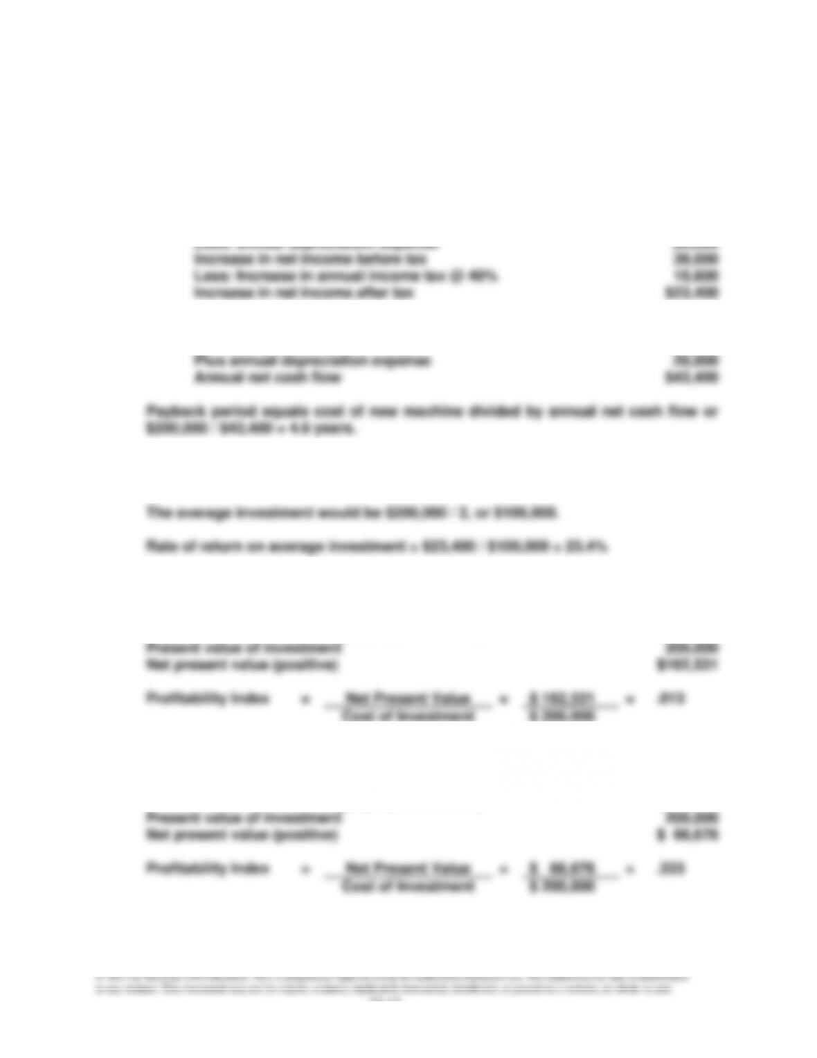
Increase in net income before tax
39,000
Less: Increase in annual income tax @ 40%
15,600
Increase in net income after tax
$23,400
Then, add back depreciation expense (noncash):
Increase in net income after tax
$23,400
Plus annual depreciation expense
20,000
Annual net cash flow
$43,400
Payback period equals cost of new machine divided by annual net cash flow or
$200,000 / $43,400 = 4.6 years.
2.
The rate of return on average investment equals the increase in net income after
tax divided by the amount of the average investment.
The average investment would be $200,000 / 2, or $100,000.
Rate of return on average investment = $23,400 / $100,000 = 23.4%
3(a)
There is a cash savings of $59,000 each year for 10 years if income taxes are
ignored. The present value factor for a 10-year annuity at 10% is 6.1446.
Present value of cash savings ($59,000 x 6.1446)
$362,531
Present value of investment
200,000
Net present value (positive)
$162,531
Profitability Index
=
Net Present Value
=
$ 162,531
=
.813
Cost of Investment
$ 200,000
3(b)
There is a cash savings of only $43,400 each year for 10 years if income taxes are
considered.
Present value of cash savings ($43,400 x 6.1446)
$266,676
Present value of investment
200,000
Net present value (positive)
$ 66,676
Profitability Index
=
Net Present Value
=
$ 66,676
=
.333
Cost of Investment
$ 200,000